
Hands-On Numerical Derivative with Python, from Zero to Hero
Here’s everything you need to know (beyond the standard definition) to master the numerical derivative world

There is a legendary statement that you can find in at least one lab at every university and it goes like this:
Theory is when you know everything but nothing works.
Practice is when everything works but no one knows why.
In this lab, we combine theory and practice: nothing works and nobody knows why
I find this sentence so relatable in the data science world. I say this because data science starts as a mathematical problem (theory): you need to minimize a loss function. Nonetheless, when you get to real life (experiment/lab) things start to get very messy and your perfect theoretical world assumptions might not work anymore (they never do), and you don’t know why.
For example, take the concept of derivative. Everybody who deals with complex concepts of data science knows (or, even better, MUST know) what a derivative is. But then how do you apply the elegant and theoretical concept of derivative in real life, on a noisy signal, where you don’t have the analytic equation?
In this blog post, I would like to show how a simple concept like a derivative can underline much complexity when dealing with real life. We would do this in the following order:
- A very brief introduction to the concept of derivative, symbolic derivative, and numeric derivative
- Implementation of the numerical derivative concept and limitation
- Refinements of the numerical derivative to overcome the simple implementation limitations.
Let’s get into this!
1. A theoretical introduction of Derivatives
I am sure that the concept of derivative is familiar to many of you and I don’t want to waste your time: I’ll be very quick on the theoretical idea and then we’ll focus on the numerical part.
So, the derivative is the slope of the tangent line of a curve. For example, the derivative is the slope of the orange line at point x = 2 for the curve y = x² .
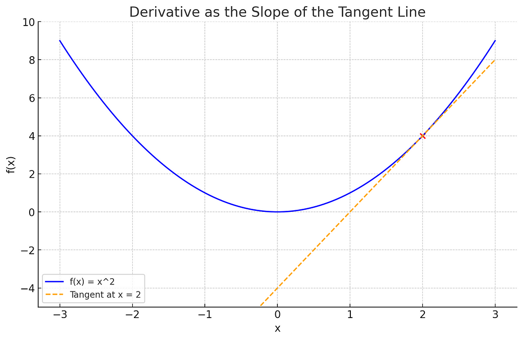
Now, a large positive derivative means that you are rapidly increasing at that point: if you increase the x, then you are going to increase y. All is summarized in this powerful definition:

That’s it. That’s the last theoretical bit of this article, I promise. Let’s do the real thing now.
2. Introduction to the numerical implementation
When we have the symbolic representation of an equation, everything is very simple. For example, we do know (from theory) that:

But let’s say we do not have the symbolic equation. How do we compute the derivative?
Well, in real life (with a numeric signal) you don’t have the luxury to take “h that tends to 0”. The only thing you have is:
- A signal: that is a list of values.
- The “time” axis: another list of values
Surely none of these two (neither the signal nor the time axis) are continuous. So your only hope is to do something like this:
def dydx(y,x,i):
return (y[x[i]]-y[x[i+1]])/(x[i+1]-x[i])
Meaning that you can’t really do “less than 1 step” in the discrete space. So you might think: “ok then, let’s do that! Let’s consider h as 1 and move 1 step at a time”
The problem is that when the signal is noisy the derivative might be incredibly large not because the signal is really increasing on the x direction, but just because it happens to increase because of the noise.
Think of an up and downy signal like this:
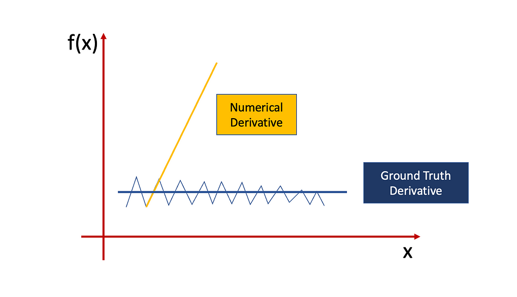
The derivative is extremely unstable but the signal is not increasing or decreasing anywhere. It is changing locally, but it’s just a random variation of the noise that we are not interested in.
So what do we do in those cases? Let’s see it together:
2.1 The simple implementation and its limitations:
Let’s explore a real case and let’s do it in Python. For this blogpost you don’t need a lot, I used sklearn, scipy, numpy, and Matplotlib. They might all be in the Anaconda package (it’s hard to keep track on it) but if not a simple pip install would do the trick.
Anyways, let’s import them:
Now let’s consider a very very simple quadratic signal.
The numerical derivative can be done using numpy and:
np.diff(y)/step
Where “step” would be “h” and, in this case, is the distance between the second and the first x. So if we do “theoretical vs numerical” we get something like this:
So it works well, let’s wrap up the article (I’m kidding)
The problem comes when the signal is not the fairy tale signal but it is one that comes from the real world. When the data comes from the real world they will necessarily have noise. For example, let’s consider the same previous signal but let’s make it a tiny bit noisier.
This is the slightly noisy signal:
It’s noisy but it’s not THAT noisy, right? HOWEVER, the derivative is completely messed up by this very small noise.
So how are we going to fix this? Let’s see some of the solutions.
3. Derivative Refinement
3.1 Cleaning the signal
The first thing we could do (the easier) is to smooth the original signal: if we know our signal is noisy, we should try to reduce the noise before doing anything else.
My favorite way to reduce noise is the Savitzky-Golay filter (I talk about it in another article you can find it here).
Let’s smooth the signal and see how it looks like:
Now we can do the derivative on the smoothed signal:
MUCH better. Nonetheless, this is not really a derivative refinement. This is more like applying the same concept to a smoothed signal. A little bit of cheating, but it’s a first step. Let’s do some more refinement.
3.2 Custom step size
From a theoretical point of view, the smaller the h is, the better it is. Nonetheless, if the signal is noisy, we might consider h as a parameter. So we can tune this parameter and see how the derivative looks like.
For example, if the x axis is between -2 (seconds for example) and 2 seconds with step = 0.004 seconds, then we might think that we can compute the derivative after 0.4 seconds (100 points) rather than after 0.004 seconds (1 point).
In order to do that we have to define our own numerical derivative function. Just like this*:
*We need to be careful because at the end of the signal we will have that we don’t have anymore 100 points but like 20, or 30. So I made a little check that if we get less than half of what you have in the beginning you stop computing the derivative
Let’s test this method again:
And let’s modify the definition of the derivative.
So our “windowed” version of the derivative is way better than the derivative on the smoothed signal (first refinement).
3.3 Custom step size + Linear Regression
Now, modifying the step size helps, but it might not be enough. Let’s consider this case.
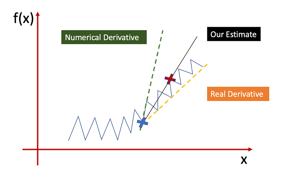
If we want to compute the derivative of f(x) for the point = blue cross we have, so far, two alternatives:
- Green line, we just trust the next point and do the tangent line
- You do the windowed approach we proposed (black line)
As we can see, the windowed approach is similar to the orange (real) ground truth, but it is not quite there. This is because, if the noise preserves, we will have a little bit of noise even after k steps. So how can we fix that?
Well, instead of considering the difference between blue and red crosses only, and then normalizing it with the x difference, we can run the Linear Regression algorithm between ALL the points between blue and red cross.
By applying the linear regression we are actively considering the tangent line (line that passes between blue and red point) but we are also incorporating all the other points in the middle. This means that we don’t just blindly trust the red cross, but we consider everything that is in between, thus averaging on the noise. Of course, once we do the linear regression, the corresponding “derivative” is the coefficient (or slope) of the fitted line. If you think about it, at the extreme limit, if you only have two points the slope of the fitted linear regression is exactly the definition of derivative.
So in a few words: we keep doing our derivative by “windowing” BUT we apply the linear regression method as well.
The effect of this (spoiler) is to efficiently smooth the derivative of the signal, as we expected.
I really like this estimation of the derivative so let’s test it with an hardcore case, i.e. a very noisy signal:
So we are going to test the two methods:
- Windowed Derivative on the Filtered Signal
- Windowed Linear Regression Derivative on the Filtered Signal
First let’s implement number 2:
These are the implemented methods:
As we can see, the orange and red estimate of the derivatives are similar but the red estimate is smoother, making the derivative less noisy. So we can consider this refinement as better than the previous refinement.
4. Conclusions
There we are, many derivatives versions later :)
In this blogpost, we talked about derivatives. In particular, we did the following:
- We described the theoretical definition of the derivatives, with a very brief example on a quadratic signal.
- We defined the standard numerical definition of the derivative on a simple quadratic signal and on a noisy one. We saw that the estimate of the derivative on a noisy signal is extremely poor as it tries to “model the noise” rather than the ground truth of the signal.
- We improved the standard numerical derivative in three ways: by smoothing the signal (first method), by smoothing the signal and “windowing” the derivative (second method), by smoothing the signal, “windowing” the derivative, and applying a linear regression algorithm (third method).
- We showed how each refinement improves the previous ones, eventually getting to an efficient definition of derivatives even on noisy signals.
I really hope you appreciated this blog post and you found this interesting. ❤
5. About me!
Thank you again for your time. It means a lot.
My name is Piero Paialunga and I’m this guy here:

Image made by author
I am a Ph.D. candidate at the University of Cincinnati Aerospace Engineering Department and a Machine Learning Engineer for Gen Nine. I talk about AI, and Machine Learning in my blog posts and on Linkedin. If you liked the article and want to know more about machine learning and follow my studies you can:
A. Follow me on Linkedin, where I publish all my stories
B. Subscribe to my newsletter. It will keep you updated about new stories and give you the chance to text me to receive all the corrections or doubts you may have.
C. Become a referred member, so you won’t have any “maximum number of stories for the month” and you can read whatever I (and thousands of other Machine Learning and Data Science top writers) write about the newest technology available.
D. Want to work with me? Check my rates and projects on Upwork!
If you want to ask me questions or start a collaboration, leave a message here or on Linkedin:
piero.paialunga@hotmail.com
Hands-On Numerical Derivative with Python, from Zero to Hero was originally published in Towards Data Science on Medium, where people are continuing the conversation by highlighting and responding to this story.
from Datascience in Towards Data Science on Medium https://ift.tt/NG8lqPx
via IFTTT


