
Kickstart Your ML Journey: Scoping, Structuring, and Exploring Data (Part 1)
Kickstart Your ML Journey: Scoping, Structuring, and Exploring Data (Part 1)
A practical guide to planning and organizing your machine learning project, from data collection to exploratory analysis.

We will cover the following topics in this post
- Understand the business problem
- Set up your working environment and directory layout
- Gather data (use multithreading to speed up 2 to 4x)
- Pre-process data (use vectorization to speed up 10x)
- Gain valuable insights through EDA
- Build interactive visualizations (in Part 2 of this series)
- Finally use ML to answer questions (in Part 3 of this series)
- Extras: you will also learn how to modularize the code into independent and reusable components, as well as how to use abstraction.
Note: this post is intended for beginner to mid level data scientists.
Almost all data science and ML projects start with a business problem. So, let’s define the problem that we are trying to solve here first.
Say, you work for a taxi service company in NYC and your team is trying to allocate resources (drivers), and set prices to maximize profits and customer satisfaction. To come up with the solution, you and your team divide this problem into several sub-problems:
- Identify the maximum drivers the company can allocate constrained by the budget.
- Identify the movement of people (in taxis) across the city at different times.
- Identify the demand for taxi at different times in different parts of the city (where are the hot spots?).
- Predict how much time it takes for a taxi to complete a trip from location A to B at a given time of the day.
- Optimize the allocation to fit the budget constraint and meet the demand at all times.
Say, you were asked to come up with insights on the 2nd and 3rd problems, and build a ML model to solve the 4th problem, i.e. predict the taxi trip duration from location A to B at a given time of the day.
Define the KPIs for the project
Discuss with the stakeholders to define the success criteria for the tasks given to you. Say, you come up with the following:
- Build interactive visualization and basic stats to gain insights into the traffic patterns, hot spots, etc. (2nd and 3rd)
- Build a prediction model such that the predicted time is +-5 minutes of the actual time 90% of the times. (4th) i.e. given the date and time of the trip and the pickup and drop-off locations, predict the trip duration.
Now you are all set to hop on your tasks. You should set up weekly cadence meetings with the stakeholders to share your progress and get regular feedback to ensure success. Depending on the company and team you work with, you may have to participate in regular sprints.
Link to Github repo. EDA notebook covered in this post.
Identify data source
Enough talk. Let’s just get that data and begin the work. After thorough research, you find that there exists a large open-source dataset for taxi trips. NYC Taxi & Limousine Commission (TLC) has made Trip Record Data available for all years starting 2009. Note: Always make sure to check the license of use before using the data. For this project, assume that the data was generated and is owned by your company.
Note about the taxi data license
The data from the New York City Taxi and Limousine Commission (TLC) Trip Record Data website is available to the public under the Open Data Commons Open Database License (ODbL). This license allows for the use, sharing, and modification of the data as long as attribution is given to the original source and any derivative works are also licensed under the ODbL.
Terms of use: http://www1.nyc.gov/home/terms-of-use.page
Citation: https://www1.nyc.gov/site/tlc/about/tlc-trip-record-data.page
Create your EDA and ML environment
It is always recommended to have a separate virtual environment for each project — to make sure you don’t mix or break dependencies and your work is easily reproducible. You can refer to this link to understand more about virtual environments. I will show you how to create one with conda:
- Note: for dev work on my local machine, I use VSCode for editing python scripts and other docs like readme, etc.; and Jupyter Lab for experimentation, editing and running Jupyter notebooks. I personally find this combination best for my data science and ML development work. ** see note below
- Next, you will need a package manager like `conda`. If you don’t worry about storage space and want all the basic libraries pre-installed, then install Anaconda. But if you want to download the bare minimum and don’t mind installing the basic dependencies later yourself, I’d suggest go with the lighter version Miniconda. Make sure to install the correct versions for your OS.
**Note: The process I follow while working on a data science project is:
- Try the code in jupyter notebook first.
- Once everything is working as expected, start moving the main components of the code to .py files, and just import those modules in the notebook.
- This way, you are preparing reusable components of the code, and also making it easier for the code to be put in production later. (trust me, this is very helpful)
You can follow along the Readme file to setup the conda evironment.
Download the data and gain higher level insights
Information on how to extract the data from city of new York’s website can be found here (2016 data).
Say you are focusing on year 2016. The total number of yellow taxi rides for the year of 2016 was around 131M; but for the sake of working on a local machine let’s extract only a fraction of the data. Let's extract 700,000 trip records (randomly) from each month from January to June of 2016 i.e. we will extract only 4.2M rides out of the total 131M. And extracting the first 6 months only because only the first 6 months have the exact pickup and dropoff lat lon locations (the later ones have taxi zone info only).
Since this is an I/O job, we will use multithreading to reduce the overall time of data fetch.
# A glimpse into the raw data
<class 'pandas.core.frame.DataFrame'>
RangeIndex: 4200000 entries, 0 to 4199999
Data columns (total 10 columns):
 #   Column              Dtype
---  ------              -----
 0   vendorid            int64
 1   pickup_datetime     datetime64[ns]
 2   dropoff_datetime    datetime64[ns]
 3   passenger_count     int64
 4   trip_distance       float64
 5   pickup_longitude    float64
 6   pickup_latitude     float64
 7   store_and_fwd_flag  object
 8   dropoff_longitude   float64
 9   dropoff_latitude    float64
dtypes: datetime64[ns](2), float64(5), int64(2), object(1)
memory usage: 320.4+ MB
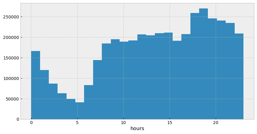
# Below is a histogram of taxi trips taken across the entire day.
# We can see a dip in the night and early morning hours as would be expected.
_ = plt.hist(nyc_sql['dropoff_datetime'].dt.hour, bins = 24)
Since we want to predict the trip_duration (y variable), that will be our dependent variable. All other variables will be independent variables (X) which affect the trip_duration .
Note: We need to remove the trip_distance column because it is strongly associated with our dependent variable trip_duration, and using that for prediction will mean allowing data leakage. And we won’t have the trip_distance data for a fresh test set anyways.
Pre-process, add features to data, EDA
Next we will add some features to the dataset and at the same time also clean it, and remove outliers, which I have defined as below:
- trip_duration < 60 seconds OR trip_duration > 99.8th percentile value of the trip_duration in the data
- The pickup and dropoff latitudes and longitudes should be within the NYC boundary defined as nyc_long_limits = (-74.257159, -73.699215), nyc_lat_limits = (40.471021, 40.987326))
- haversine_distance (add link) between the pickup and dropoff points. Trim it to > 0 and < its 99.8th percentile value.
- We will also add new features and remove outliers after some EDA based on our observations.
# Fraction of data omitted by cleaning = 2.70 %,
# dataset reduced from 4,200,000 to 4,086,468
The features are self-explanatory so I won’t describe them here. Note that the datetime features like month, hour, weekday, etc. have been defined based on the pickup datetime only, assuming most trips are within the same month, hour and day.
The target variable trip_duration was obtained by subtracting the drop-off_datetime from pickup_datetime (units: seconds).
<class 'pandas.core.frame.DataFrame'>
RangeIndex: 4086468 entries, 0 to 4086467
Data columns (total 17 columns):
 #   Column              Dtype
---  ------              -----
 0   vendorid            int64
 1   pickup_datetime     datetime64[ns]
 2   dropoff_datetime    datetime64[ns]
 3   passenger_count     int64
 4   pickup_longitude    float64
 5   pickup_latitude     float64
 6   store_and_fwd_flag  object
 7   dropoff_longitude   float64
 8   dropoff_latitude    float64
 9   trip_duration       float64
 10  pickup_date         datetime64[ns]
 11  pickup_month        int64
 12  pickup_day          int64
 13  pickup_hour         int64
 14  pickup_weekday      category
 15  holiday             int64
 16  distance_hav        float64
dtypes: category(1), datetime64[ns](3), float64(6), int64(6), object(1)
memory usage: 502.7+ MB
→ Some stats about our target variable trip_duration

~65% of the trips were between 5 to 20 minutes. And almost 95% were between 1 to 40 minutes.
Note: The widths of the bars are shown equal in the above chart for simplicity, but they are not actually equal. For example, 5–10 is 5 minutes width apart, but 10–20 is 10 minutes width apart.
Some stats on the calculated haversine distance (in the notebook I have also compared this estimation to the removed actual trip distance).
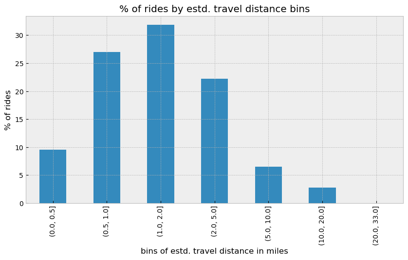
~83% of the trips were between 0.5 to 5 miles. 75% of the trips are below 3 miles.
- The calculated haversine distance values are a bit lower than the actual trip distance values, this is because the haversine distance calculates the distance along the curvature of the earth on a straight path which will always be shorter than the actual path. But it’s a good approximation nevertheless as we cannot use the actual trip distance values.
I have also calculated the average speed (mph) of each trip, by
nyc_raw['speed_mph'] = nyc_raw.distance_hav/(nyc_raw.trip_duration/60/60)
99% of the trips had an average speed below 25 mph. If you have ever driven in NYC then you know this is True.
More EDA
Let’s plot a scatter plot showing the pickup and drop-off points on a X-Y axis.

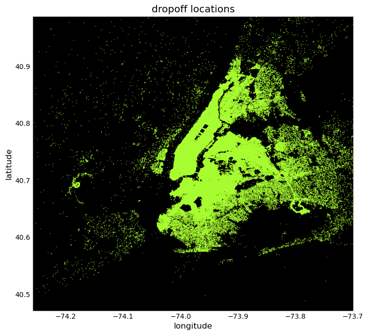
- The scattered points give out the overall layout of the NYC boroughs and we can see that the density is highest in the Manhattan area, especially for the pickups. The dropoff locations are more spread out.
- Pickups and Dropoffs are denser in the John F. Kennedy International Airport area whereas only dropoffs are denser in the Newark Liberty International Airport area because the Newark airport is served majorly by the Newark taxis and not by NYC taxis.
- LaGuardia Airport also seems to be served well by the yellow taxis.
Also, since the yellow (medallion) taxis are able to pick up passengers only in the five boroughs of NYC, the pickup locations are mostly within NYC but the dropoffs can be outside the limits as seen from the plots.
→ Let’s plot the trip duration and count of trips variation across the day
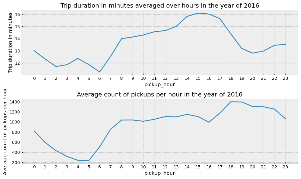
- Note: Please notice that the y-axis doesn’t start at 0.
- As one would expect the trip duration and the number of rides are higher in the evening time. As the number of rides go up in a certain area one can expect the resulting traffic to increase the trip duration time.
- From the 2nd plot we can see how the pickup rides increase steadily from 5am to 8am only to flatten out between 8am to 4pm and then again steeply increase from 4pm to 6pm to fall down later.
- The average trip duration is around 15 minutes during the evening time.
Distribution of estimated distance — grouped by trip duration

- The distribution of distance is narrow and located between 0 to 7 miles for the shorter trips from 0 to 20 minutes as expected.
- As the trip_duration bins go higher the distance distributions shift to the right because trip duration is directly proportional to the distance travelled.
- The >20 and <60 trip duration bins have a wide spread of distance values with multiple peaks, wheras the 60–100 bin has the distance distribution between 10 to 15 miles indicating long trips. The two peaks in the 20–40 and 40–60 trip_duration bins can indicate that there are other factors that affect the trip duration but it also can mean that our estimated distance values are lower than the real values especially for the lower peaks.
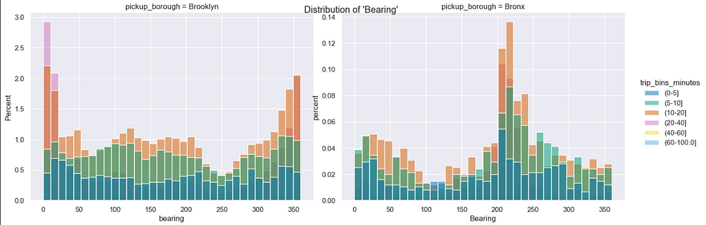
Distribution of trip direction (bearing) — grouped by trip duration
(0 -> North, 90 -> East, 180 -> South, 270 -> West)
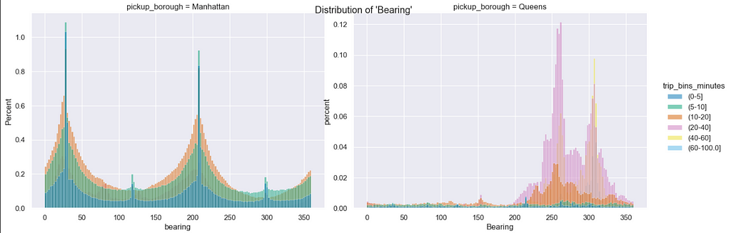
- Most of the trips from Queens are directed towards West and North-West. This kind of makes sense because La Guardia airport lies in the North West (of Queens) and also if a taxi has to travel from Queens to Manhattan it has to travel in the West direction.
- Trips from Brooklyn seem to be spread out uniformly across all directions but most common direction is North (0 Deg and 360 Deg) which indicates travel to Manhattan.
- Trips from Bronx (with higher trip duration) are also directed mostly in the South-West direction indicating travel to Manhattan.
- In the next blog post (Part 2) we will:
- Add taxi zones information to the dataset and break down some duration stats by taxi zones.
- Build an interactive visualization for the stakeholders to play with, and see how the trip duration value changes across the different parameters like — pickup and drop-off zones, day of week, hour of day, etc.. (shown at the top of this post)
2. And in the 3rd post, we will build ML models to predict the taxi trip duration from point A to B.
Kickstart Your ML Journey: Scoping, Structuring, and Exploring Data (Part 1) was originally published in Towards Data Science on Medium, where people are continuing the conversation by highlighting and responding to this story.
from Datascience in Towards Data Science on Medium https://ift.tt/TzD8aY9
via IFTTT


