
Make Your Way from Pandas to PySpark
Learn a few basic commands to start transitioning from Pandas to PySpark

Introduction
I am part of a few data science communities on LinkedIn and from other places and one thing that I see from time to time is people questioning about PySpark.
Let’s face it: Data Science is too vast of a field for anyone to be able to know about everything. So, when I join a course/community about statistics, for example, sometimes people ask what is PySpark, how to calculate some stats in PySpark, and many other kinds of questions.
Usually, those who already work with Pandas are especially interested in Spark. And I believe that happens for a couple of reasons:
- Pandas is for sure very famous and used by data scientists, but also for sure not the fastest package. As the data increases in size, the speed decreases proportionally.
- It is a natural path for those who already dominate Pandas to want to learn a new option to wrangle data. As data is more available and with higher volume, knowing Spark is a great option to deal with big data.
- Databricks is very famous, and PySpark is possibly the most used language in the Platform, along with SQL.
In this post, we will learn and compare the code snippets for Pandas and PySpark for the main wrangling functions:
- Summarizing
- Slicing
- Filtering
- Grouping
- Replacing
- Arranging
Let’s dive in.
Preparing the Environment
For the sake of simplicity, we will use Google Colab in this exercise.
Once you open a new notebook in the tool, install pyspark and py4j and you should be good to go.
!pip install pyspark py4j
These are the modules we need to import. We will import SparkSession, the functions module, so we can use methods like mean, sum, max, when etc. For the Python side, just pandas and numpy.
# import spark and functions
from pyspark.sql import SparkSession
from pyspark.sql import functions as F
from pyspark.sql.functions import col, mean, count, when

# Imports from Python
import pandas as pd
import numpy as np
Since we are working in a Jupyter Notebook, a Spark session needs to be initialized before you can use it. Notice that, if you’re using Databricks to code along (Community edition — free), the spark session is already initiated with the cluster and you won’t need to do that. But in Colab, we need this line of code.
# Create a spark session
spark = SparkSession.builder.appName("tests").getOrCreate()
This is the dataset to be used: California Housing, a sample dataset under the Creative Commons license.
Pandas vs PySpark
The drill now will be presenting each code snippet and commenting on the differences between both syntaxes.
Load and View Data
To load data, both syntaxes are pretty similar. While in Pandas we use the pd alias, in Spark we use the name of the Spark Session, in our case, we named it spark. I recommend you use this name as a default, since many tutorials will give you code snippets with spark as the name of the Spark session.
Pandas use the snake_case with underscore, and Spark will use the dot ..
# Load data with Pandas
dfp = pd.read_csv(pth)

# View data
dfp.head()
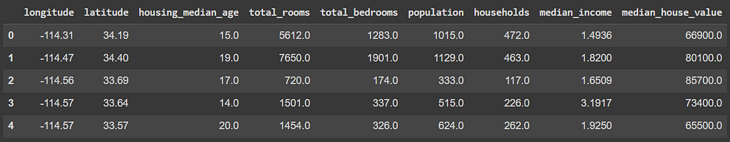
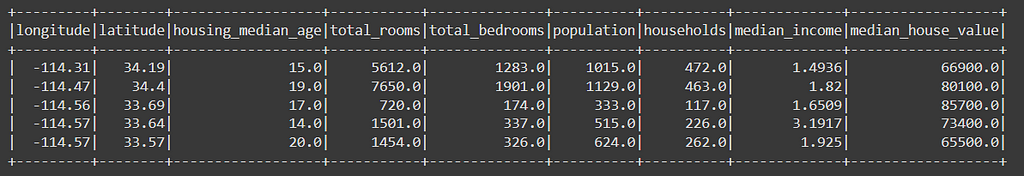
Additionally, in Spark the (schema) variable type inference is not always automatic, so use the argument inferSchema=True.Now, let us load and view data with Pyspark. The .limit(n) method will limit the result to the number n of rows we want to display.
# Load data to session
df = spark.read.csv(pth, header=True, inferSchema=True)

# Visualizing the Data
df.limit(5).show()
Summarizing
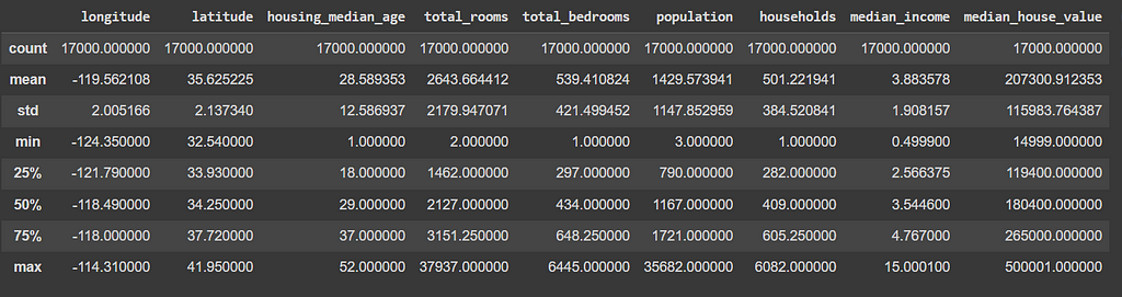
The next comparison is the summarization. Usually, an easy way to summarize the statistics of a dataset is using the .describe() method. In Spark, the method is the same.
This is Pandas.
# Summarizing Data in Pandas
dfp.describe()
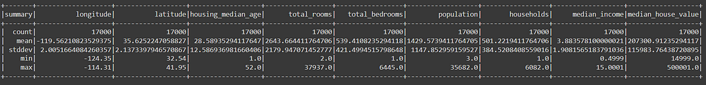
However, notice that Spark brings less information. The percentiles are not displayed. This is possibly because it is meant to work with a lot of data, so simplifying the output mean less calculations, what should make it faster.
# Summarizing Data with Spark
df.describe().show()
The next snippet will display the percentiles of the data, in case you want to see it.
# Percentiles Spark
(df
 .agg(*[F.percentile(col, [.25, .5, .75]) for col in df.columns])
 .show()
 )
Slicing
Slicing is cutting the dataset to see a specific part of it. It is different than filtering because it does not carry conditions, though.
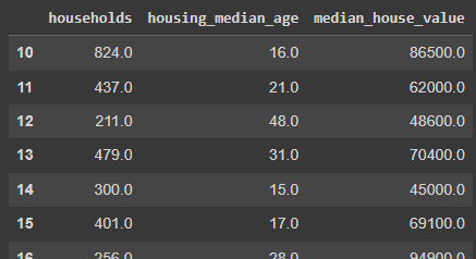
In Pandas, the code is as follows. Using .loc[row,col] we can determine the row numbers and columns to display.
# Slicing (Selecting) Data in Pandas
dfp.loc[10:20, ['households', 'housing_median_age', 'median_house_value']]
Be aware that in Spark you can’t directly slice a data frame by rows, knowing that it is not indexed like Pandas.
Spark Dataframes are not row-indexed like Pandas.
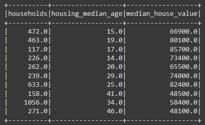
As you start using Spark, you will notice that its syntax is very influenced by SQL. So, to slice the data, we will select() the columns we want to see from the data.
# Slicing in Spark
(df # dataset
 .select('households', 'housing_median_age', 'median_house_value') #select columns
 .limit(10) # limit how many rows to display
 .show() #show data
)
The next code adds the row number column and the ability to slice by row. However, this is an intermediate-level code for PySpark, using the Window functions. I will leave it here, and you can learn more with a link from the References section.
from pyspark.sql.window import Window
from pyspark.sql.functions import row_number

# Slicing by columns and rows in Spark
(df # dataset
 .select('households', 'housing_median_age', 'median_house_value') #select columns
 .withColumn('row_n', row_number().over(Window.orderBy('households'))) #create row number column
 .filter( col('row_n').between(10,20) ) #slice by row number
 .show() #show data
)
Filtering
The filters allow us to show only rows and columns that follow certain conditions.
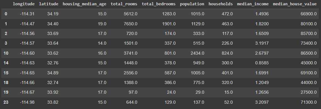
In Pandas, I prefer to use the .query() function. It is much more intuitive and easy to use. But, of course, you can use the good-old slicing notation as well.
# Filtering data Pandas
dfp.query('housing_median_age < 20').head(10)
The code snippet is filtering on houses with less than 20 years since construction.
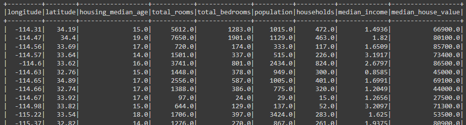
In Spark, the method to filter can be .filter() or it can be .where() (like in SQL). Within the filter function, you can add the col('col_name') and condition, like < 20 in the example. To add other conditions, just use & for AND and | for OR.
Note: in Spark, every time we will apply a transformation or a function to a column, we must use the col() function to make it an object. For example, here we are applying a condition to the column, thus the need to use col.
# Filtering in Spark
(df #dataset
 .filter(col('housing_median_age') < 20) # Filter
 .show() #display data
 )
Grouping
Now, getting to one of the most used wrangling functions, the group by, that allows us to aggregate data.
In Pandas, we can write using the slicing notation, as well as we can use the dictionary style, which is similar to the Spark syntax.
# Grouping in Pandas
(dfp
 .groupby('housing_median_age')
 ['median_house_value'].mean()
 .reset_index()
 .sort_values('housing_median_age')
 .head(10)
)

# Get different aggregation values for different variables
(dfp
 .groupby('housing_median_age')
 .agg({'median_house_value': 'mean',
       'population':'max',
       'median_income':'median'})
 .reset_index()
 .sort_values('housing_median_age')
 .head(10)
 )
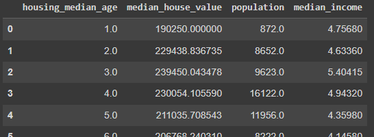
And next is the Spark Code. Notice how the second snippet is very similar to the Pandas' syntax with a dictionary.
Another observation is that for the mean() function we are not using F.mean, but we use it for F.max and F.median. The reason is because all the wrangling functions are in the module pyspark.sql.functions.
At the beginning of our code, we imported mean separately ( from pyspark.sql.function import mean)and the others we just imported as from pyspark.sql import functions as F. So, we must call F. for those not imported separately. This rule is just like regular module importing rules in Python code.
# Grouping in Spark
 (df #dataset
 .groupBy('housing_median_age') #grouping
 .agg(mean('median_house_value').alias('median_house_value')) #aggregation func
 .sort('housing_median_age') #sort
 .show()#display
)

# Grouping different variables in Spark
(df #dataset
 .groupBy('housing_median_age') #grouping
 .agg(mean('median_house_value').alias('median_house_value'), #aggregation funcs
      F.max('population').alias('population'),
      F.median('median_income').alias('median_income'))
 .sort('housing_median_age') #sort
 .show() #display
)
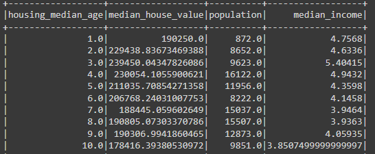
Another comment to make is that aggregation functions in PySpark will change the variable name in the output. So, for example, the name of the output would be mean('median_house_value') if we had not used the .alias() function to rename the output column.
Replacing
To replace values, there are different ways to do that using Pandas. In the next code, we are using a combination of .assign and .where.
# Replacing values in Pandas
(dfp #dataset
 .assign(housing_median_age=
         dfp['housing_median_age'].where(dfp.housing_median_age > 15,
         other="potential buy") ) #assign replaced values to variable
 )
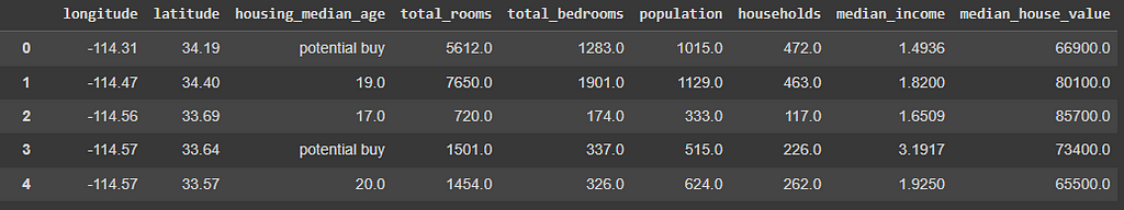
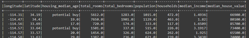
Using Spark, an easy way to do that is by rewriting the column (or adding a new one) using the conditions within the .when function from Spark. The code below rewrites the housing_median_age column using a .when function that replaces houses up to 15 years of age with the word “potential buy”, otherwise it just repeats the current value.
# Replace values in Spark
(df #dataset
 .withColumn('housing_median_age',
                when(col('housing_median_age') <= 15, 'potential buy')
                .otherwise(col('housing_median_age'))
                ) #new column
 .show() #display
)
Arranging
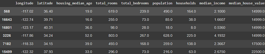
Finally, arranging data is just ordering it. In Pandas, we can do that using sort_values().
# Arrange values in Pandas
(dfp
 .sort_values('median_house_value')
 .head(10)
)
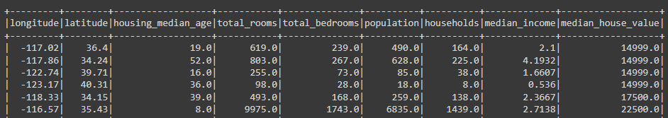
Using Spark, the only difference is the function orderBy() replacing the sort_values. If we want to order descending, we can add the column indicator function and the descending function, like this col('col_name').desc().
# Arrange values in Spark
(df #dataset
 .orderBy('median_house_value') #order data
 .show() #display
)

# Arrange values in descending order
(df
 .orderBy(col('median_house_value').desc())
 .show()
)
Before You Go
That’s a wrap.
In this post, we have compared the main wrangling functions using Pandas and Pyspark and commented on their syntax differences.
This is useful for those starting their journey learning PySpark to wrangle big data. Remember, Spark is not difficult. If you already work with Python, the syntax is very easy to catch.
People who know SQL code and Python will see a lot of influence of the SQL language in the PySpark methods. Those who already like Polars will benefit the most from knowledge transfer, given that both Polars and PySpark share many similarities in syntax.
Learn More
Interested in learning more about PySpark?
Well, lucky you, because I have a whole online course in Udemy and I am applying a coupon code to offer you the best price possible through this link.
Contacts
If you liked this content, follow me for more.
Also, let’s connect on LinkedIn.
Code
You can find the code from this exercise in this GitHub repo:
https://github.com/gurezende/Studying/blob/master/PySpark/PySpark_in_Colab.ipynb
References
- How to Replace Values in Pandas
- Functions - PySpark 3.5.3 documentation
- DataFrame - pandas 2.2.3 documentation
- PySpark Window Functions
- Pandas Query: the easiest way to filter data
Make Your Way from Pandas to PySpark was originally published in Towards Data Science on Medium, where people are continuing the conversation by highlighting and responding to this story.
from Datascience in Towards Data Science on Medium https://ift.tt/hiWj1tq
via IFTTT
