Start Asking Data Why | Causality Intro| Eyal Kazin
Start Asking Your Data “Why?” — A Gentle Intro To Causality
A beginner’s guide to thinking beyond correlations.
“Causation is not merely an aspect of statistics — it is an addition to statistics” — Judea Pearl

Correlation does not imply causation. It turns out, however, that with some simple ingenious tricks one can, potentially, unveil causal relationships within standard observational data, without having to resort to expensive randomised control trials.
This post is targeted towards anyone making data driven decisions. The main takeaway message is that causality may be possible by understanding that the story behind the data is as important as the data itself.
By introducing Simpson’s and Berkson’s Paradoxes, situations where the outcome of a population is in conflict with that of its cohorts, I shine a light on the importance of using causal reasoning to identify these paradoxes in data and avoid misinterpretation. Specifically I introduce causal graphs as a method to visualise the story behind the data point out that by adding this to your arsenal you are likely to conduct better analyses and experiments.
My ultimate objective is to whet your appetite to explore more on causality, as I believe that by asking data “Why?” you will be able to go beyond correlation calculations and extract more insights, as well as avoid common misjudgement pitfalls.
Note that throughout this gentle intro I do not use equations but demonstrate using accessible intuitive visuals. That said I provide resources for you to take your next step in adding causal inference to your statistical toolbox so that you may get more value from your data.
The Era of Data Driven Decision Making
“In [Deity] We Trust, All Others Bring Data!” — William E. Deming
In this digital age it is common to put a lot of faith in data. But this raises an overlooked question —
Should we trust data on its own?
Judea Pearl, who is considered the Godfather of causality, articulated best:
“The collection of information is as important as the information itself “ — Judea Pearl
In other words the story behind the data is as important as the data itself.
This manifests in a growing awareness of the importance of identifying bias in datasets. By the end of this post I hope that you will appreciate that causality pertains the fundamental tools to best express, quantify and attempt to correct for these biases.
In causality introductions it is customary to demonstrate why “correlation does not imply causation” by highlighting limitations of association analysis due to spurious correlations (e.g, shark attacks 🦈 and ice-cream sales 🍦). In an attempt to reduce the length of this post I defer this aspect to an older one of mine. Here I focus on two mind boggling paradoxes 🤯 and their resolution via causal graphs to make a similar point.
Paradoxes in Analysis
To understand the importance of the story behind the data we will examine two counter-intuitive (but nonetheless true) paradoxes which are classical situations of data misinterpretation.
In the first we imagine a clinical trial in which patients are given a treatment and that results in a health score. Our objective is to assess the average impact of increased treatment to the health outcome. For pedagogical purposes in these examples we assume that samples are representative (i.e, the sample size is not an issue) and that variances in measurements are minimal.
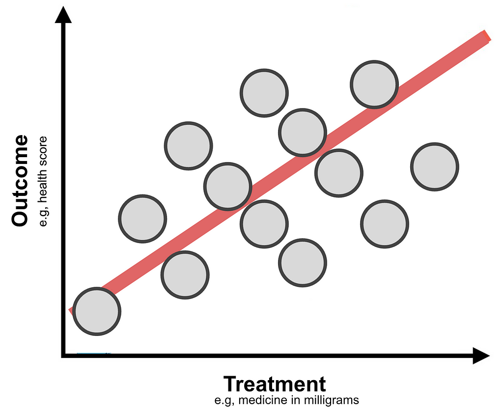
In the figure above we learn that on average increasing the treatment appears to be beneficial since it results in a better outcome.
Now we’ll color code by age and gender groupings and examine how the treatment increases impacts each cohort.
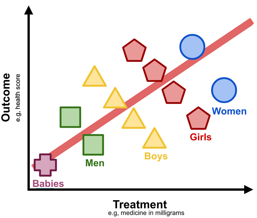
Track any cohort (e.g, “Girls” representing young females) and you immediately realise that increase in treatment appears adverse.
What is the conclusion of the study? On the one hand increasing the treatment appears to be better for the population at large, but when examining gender-age cohorts it seems disadvantageous. This is Simpson’s Paradox which may be stated:
“Trends can exist in subgroups but reverse for the whole”
Below we will resolve this paradox using causality tools, but beforehand let’s explore another interesting one, which also examines made up data.
Imagine that we quantify for the general population their attractiveness and how talented they in this figure:
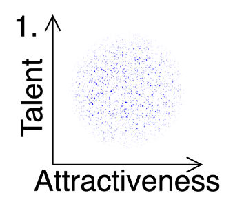
We find no apparent correlation.
Now we’ll focus on an unusual subset — famous people:
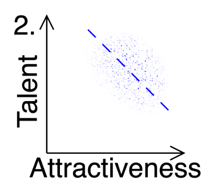
Here we clearly see an anti-correlation that doesn’t exist in the general population.
Should we conclude that Talent and Attractiveness are independent variables as per the first plot of the general population or that they are correlated as per that of celebrities?
This is Berkson’s Paradox where one population has a trait trend that another lacks.
Whereas an algorithm would identify these correlations, resolving these paradoxes requires a full understanding of the context which normally is not fed to a computer. In other words without knowing the story behind the data results may be misinterpreted and wrong conclusions may be inferred.
Mastering identification and resolution these paradoxes is an important first step to elevating one’s analyses from correlations to causal inference.
Whereas these simple examples may be explained away logically, for the purposes of learning causal tools in the next section I’ll introduce Causal Graphs.
Causal Graphs— Visualising The Story Behind The Data
“[From the Simpson’s and Berkson’s Paradoxes we learn that] certain decisions cannot be made based on the basis of data alone, but instead depend on the story behind the data. … Graph Theory enables these stories to be conveyed” — Judea Pearl
Causal graph models are probabilistic graphical models that are used to visualise the story behind the data. They are perhaps one of the most powerful tools for analysts that is not taught in most statistics curricula. They are both elegant and highly informative. Hopefully by the end of this post you will appreciate it when Judea Pearl says that this is the missing vocabulary to communicate causality.
To understand causal graph models (or causal graphs for short) we start with the following illustration of an example undirected graph with four nodes/vertices and three edges
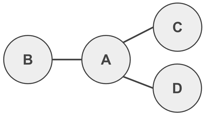
Each node is a variable and the edges communicate “who is related to whom?” (i.e, correlations, joint probabilities).
A directed graph is one in which we add arrows as in this figure
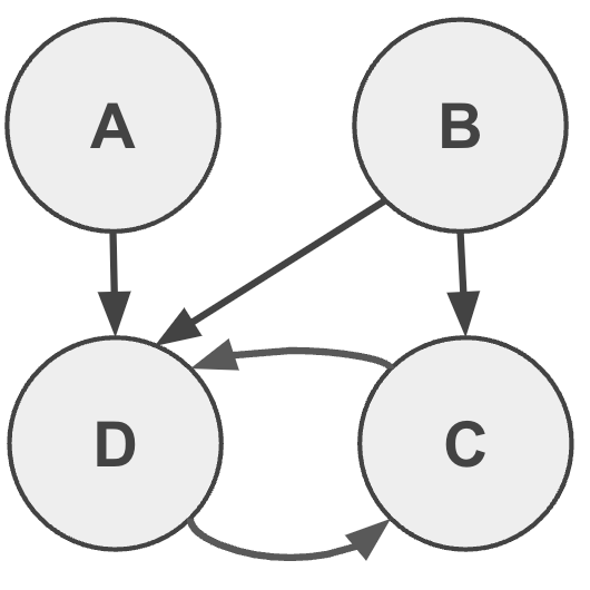
A directed edge communicates “who listens to whom?” which is the essence of causation.
In this specific example you can notice a cyclical relationship between the C and D nodes.
A useful subset of directed graphs are the directed acyclic graphs (DAG) which have no cycles as in the next figure.
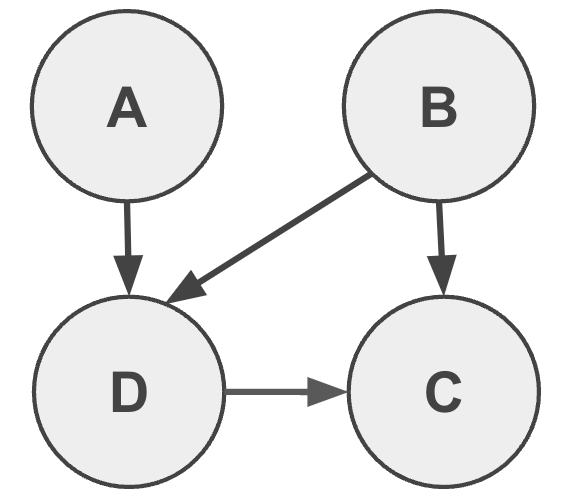
Here we see that when starting from any node (e.g, A) there isn’t a path that gets back to it.
DAGs are the go-to choice in causality for simplicity as the fact that parameters do not have feedback highly simplifies the flow of information. (For mechanisms that have feedback, e.g temporal systems, one may consider rolling out nodes as a function of time, but that is beyond the scope of this intro.)
Causal graphs are powerful at conveying the cause/effect relationships between the parameter and hence how data was generated (the story behind the data).
From a practical point of view, graphs enable us to understand which parameters are confounders that need to be controlled for, and, as we shall see, as important, which not to control for, as doing so causes spurious correlations.
The practice of attempting to build a causal graph enables
- Design of better experiments
- Draw causal conclusions (go beyond correlations by means of representing interventions, counterfactuals and encoding conditional independence relationships; all beyond the scope of this post)
To further motivate the usage of causal graph models we will use them to resolve the Simpson’s and Berkson’s paradoxes introduced above.
💊 Causal Graph Resolution of Simpson’s Paradox
For simplicity we’ll examine Simpson’s paradox focusing on two cohorts, male and female adults.
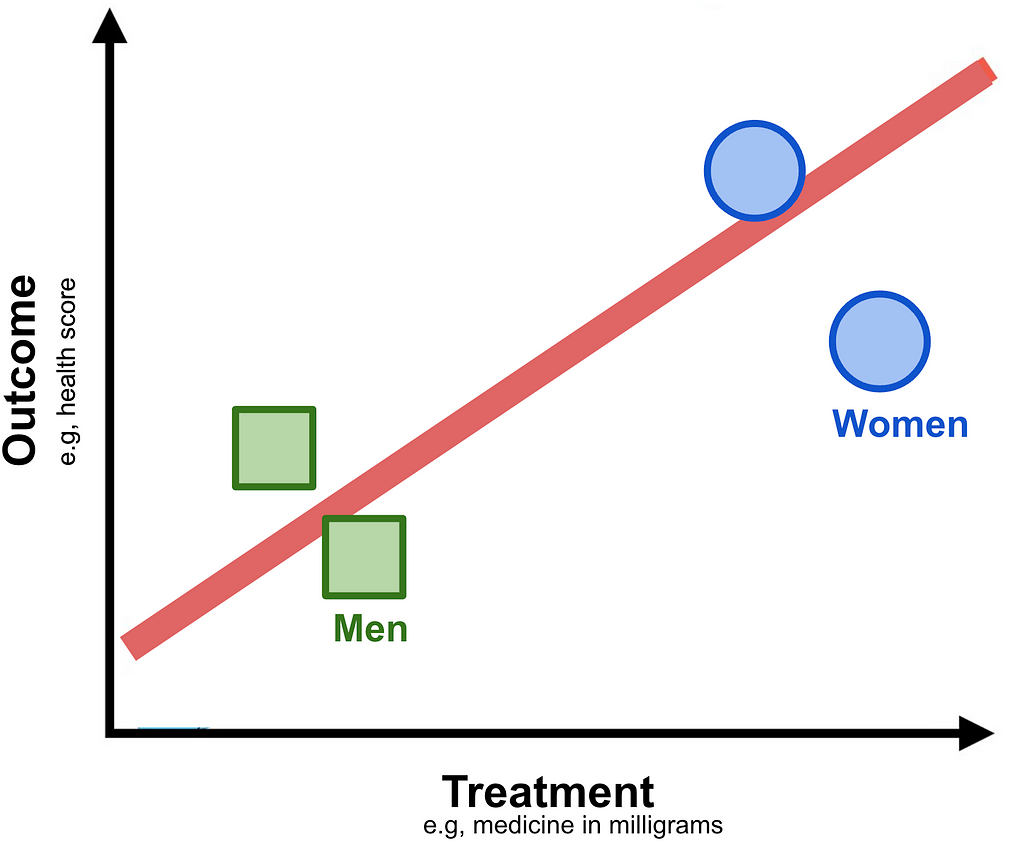
Examining this data we can make three statements about three variables of interest:
- Gender is an independent variable (it does not “listen to” the other two)
- Treatment depends on Gender (as we can see, in this setting the level given depends on Gender — women have been given, for some reason, a higher dosage.)
- Outcome depends on both Gender and Treatment
According to these we can draw the causal graph as the following
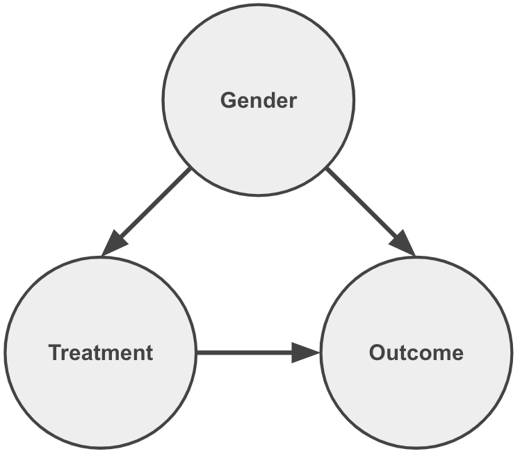
Notice how each arrow contributes to communicate the statements above. As important, the lack of an arrow pointing into Gender conveys that it is an independent variable.
We also notice that by having arrows pointing from Gender to Treatment and Outcome it is considered a common cause between them.
The essence of the Simpson’s paradox is that although the Outcome is effected by changes in Treatment, as expected, there is also a backdoor path flow of information via Gender.
The solution to this paradox, as you may have guessed by this stage, is that the common cause Gender is a confounding variable that needs to be controlled.
Controlling for a variable, in terms of a causal graph, means eliminating the relationship between Gender and Treatment.
This may be done in two manners:
- Pre data collection: Setting up a Randomised Control Trial (RCT) in which participants will be given dosage regardless of their Gender.
- Post data collection: As in this made up scenario the data has already been collected and hence we need to deal with what is referred to as Observational Data.
In both pre- and post- data collection the elimination of the Treatment dependency of Gender (i.e, controlling for the Gender) may be done by modifying the graph such that the arrow between them is removed as such:
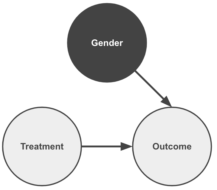
Applying this “graphical surgery” means that the last two statements need to be modified (for convenience I’ll write all three):
- Gender is an independent variable
- Treatment is an independent variable
- Outcome depends on Gender and Treatment (but with no backdoor path)
This enables obtaining the causal relationship of interest : we can assess the direct impact of modification Treatment on the Outcome.
The process of controlling for a confounder, i.e manipulation of the data generation process, is formally referred to as applying an intervention. That is to say we are no longer passive observers of the data, but we are taking an active role in modification it to assess the causal impact.
How is this manifested in practice?
In the case of the RCT the researcher needs ensure to control for important confounding variables. Here we limit the discussion to Gender (but in real world settings you can imagine other variables such as Age, Social Status and anything else that might be relevant to one’s health).
RCTs are considered the golden standard for causal analysis in many experimental settings thanks to its practice of confounding variables. That said, it has many setbacks:
- It may be expensive to recruit individuals and may be complicated logistically
- The intervention under investigation may not be physically possible or ethical to conduct (e.g, one can’t ask randomly selected people to smoke or not for ten years)
- Artificial setting of a laboratory — not true natural habitat of the population
Observational data on the other hand is much more readily available in the industry and academia and hence much cheaper and could be more representative of actual habits of the individuals. But as illustrated in the Simpson’s diagram it may have confounding variables that need to be controlled.
This is where ingenious solutions developed in the causal community in the past few decades are making headway. Detailing them are beyond the scope of this post, but I briefly mention how to learn more at the end.
To resolve for this Simpson’s paradox with the given observational data one
- Calculates for each cohort the impact of the change of the treatment on the outcome
- Calculates a weighted average contribution of each cohort on the population.
Here we will focus on intuition, but in a future post we will describe the maths behind this solution.
I am sure that many analysts, just like myself, have noticed Simpson’s at some stage in their data and hopefully have corrected for it. Now you know the name of this effect and hopefully start to appreciate how causal tools are useful.
That said … being confused at this stage is OK 😕

I’ll be the first to admit that I struggled to understand this concept and it took me three weekends of deep diving into examples to internalised it. This was the gateway drug to causality for me. Part of my process to understanding statistics is playing with data. For this purpose I created an interactive web application hosted in Streamlit which I call Simpson’s Calculator 🧮. I’ll write a separate post for this in the future.
Even if you are confused the main takeaways of Simpson’s paradox is that:
- It is a situation where trends can exist in subgroups but reverse for the whole.
- It may be resolved by identifying confounding variables between the treatment and the outcome variables and controlling for them.
This raises the question — should we just control for all variables except for the treatment and outcome? Let’s keep this in mind when resolving for the Berkson’s paradox.
🦚 Causal Graph Resolution of Berkson’s Paradox
As in the previous section we are going to make clear statements about how we believe the data was generated and then draw these in a causal graph.
Let’s examine the case of the general population, for convenience I’m copying the image from above:

Here we understand that:
- Talent is an independent variable
- Attractiveness is an independent variable
A causal graph for this is quite simple, two nodes without an edge.
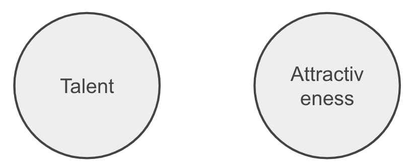
Let’s examine the plot of the celebrity subset

The cheeky insight from this mock data is that the more likely one is attractive the less they need to be talented to be a celebrity. Hence we can deduce that:
- Talent is an independent variable
- Attractiveness is an independent variable
- Celebrity variable depends on both Talent and Attractiveness variables. (Imagine this variable is boolean as in: true for celebrities or false for not).
Hence we can draw the causal graph as
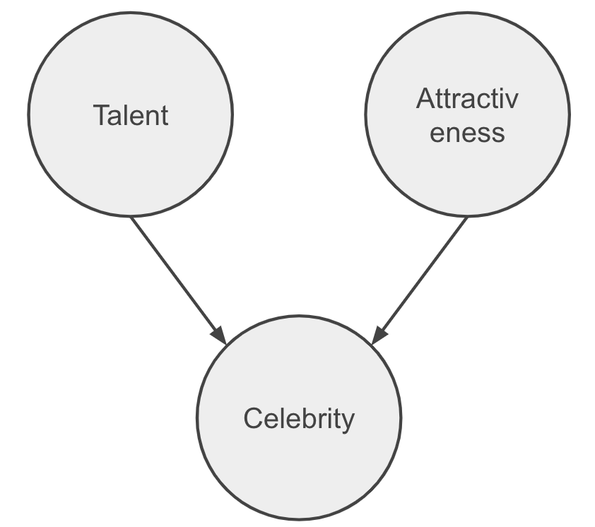
By having arrows pointing into it Celebrity is a collider node between Talent and Attractiveness.
Berkson’s paradox is the fact the when controlling for celebrities we see an interesting trend (anti correlation between Attractiveness and Talent) that is not seen in the general population.
This can be visualised in the causal graph that by confounding for the Celebrity parameter we are creating a spurious correlation between the otherwise independent variables Talent and Attractiveness. We can draw this as the following
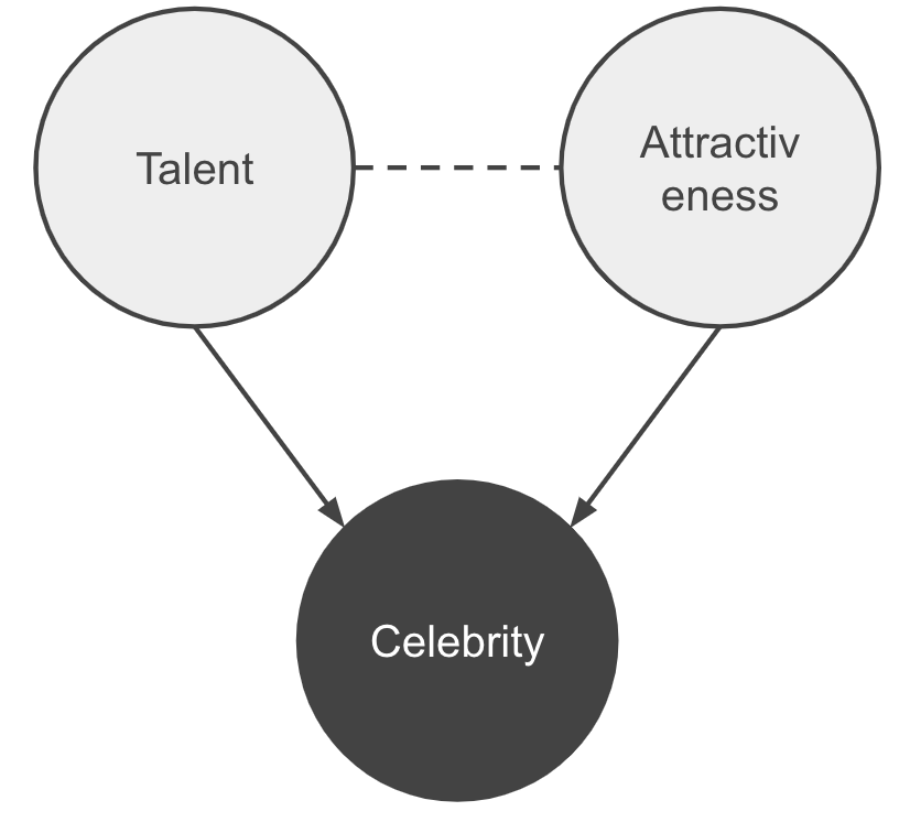
The solution of this Berkson’s paradox should be apparent here: Talent and Attractiveness are independent variables in general, but by controlling for the collider Celebrity node causes a spurious correlation in the data.
Paradoxes Summary
Let’s compare the resolution of both paradoxes:
- Resolving Simpson’s Paradox is by controlling for common cause (Gender)
- Resolving Berkson’s Paradox is by not controlling for the collider (Celebrity)
The next figure combines both insights in the form of their causal graphs
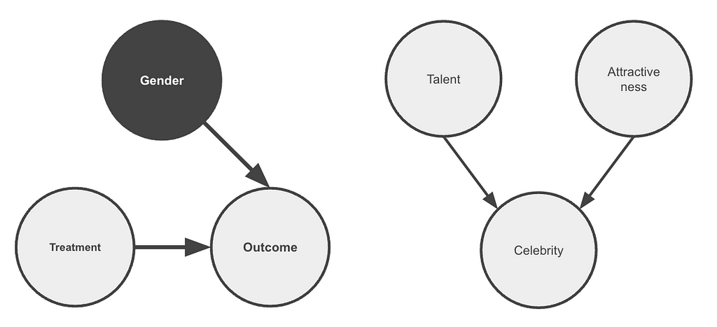
The main takeaway from the resolution of these paradoxes is that controlling for parameters requires a justification. Common causes should be controlled for but colliders should not.
Even though this is common knowledge for those who study causality (e.g, Economics majors), it is unfortunate that most analysts and machine learning practitioners are not aware of this (including myself in 2020 after over 15 years of analysis and predictive modelling experience).
``Oddly, statisticians both over- and underrate the importance of confounders” — Judea Pearl
Summary
The main takeaway from this post is that the story behind the data is as important as the data itself.
Appreciating this will help you avoid result misinterpretation as spurious correlations and, as demonstrated here, in Simpson’s and Berskon’s paradoxes.
Causal Graphs are an essential tool to visualise the story behind the data. By using them to solve for the paradoxes we learnt that controlling for variables requires justification (common causes ✅, colliders ⛔️).
For those interested in taking the next step in their causal journey I highly suggest mastering Simpson’s paradox. One great way is by playing with data. Feel free to do so with my interactive “Simpson-calculator” 🧮.
I aim to follow up with a post about causality applicability, stay tuned 📻 …
Unless otherwise noted, all images were created by the author.
Useful Resources
Here I provide resources that I find useful as well as a shopping list of topics for beginners to learn.
📚 Books

- The Book of Why — popular science reading (NY Times level)
- Causal Inference in Statistics A Primer — excellent short technical book (site)
- Causal Inference and Discovery in Python by Aleksander Molak (Packt, github) — clearly explained with python applications 🐍.
- What If? — a cohesive presentation of concepts of, and methods for, causal inference (site, github)
- Causal Inference The Mixtape — Social Science focused using Python, R and Strata (site, resources, mooc)
- Counterfactuals and Causal Inference — Methods and Principles (Social Science focused)

This list is far from comprehensive, but I’m glad to add to it if anyone has suggestions (please mention why the book stands out from the pack).
🔏 Courses

There are probably a few courses online. I love the 🆓 one of Brady Neil bradyneal.com/causal-inference-course.
- Clearly explained
- Covers many aspects
- Thorough
- Provides memorable examples
- F.R.E.E
One paid course 💰 that is targeted to practitioners is Altdeep.
💾 Software
This list is far from comprehensive because the space is rapidly growing:
- dagitty.net — a web application to construct and interpret causal graphs
- PyWhy — open source ecosystem for Causal Machine Learning (includes popular packages such as dowhy and econml).
- tigramite — Causal inference with a focus on time series data
- Causal Wizard — Causal software for effect estimation
🐾 Suggested Next Steps In The Causal Journey
Here I highlight a list of topics which I would have found useful when I started my learnings in the field. If I’m missing anything I’d be more than glad to get feedback and adding. I bold face the ones which were briefly discussed here.
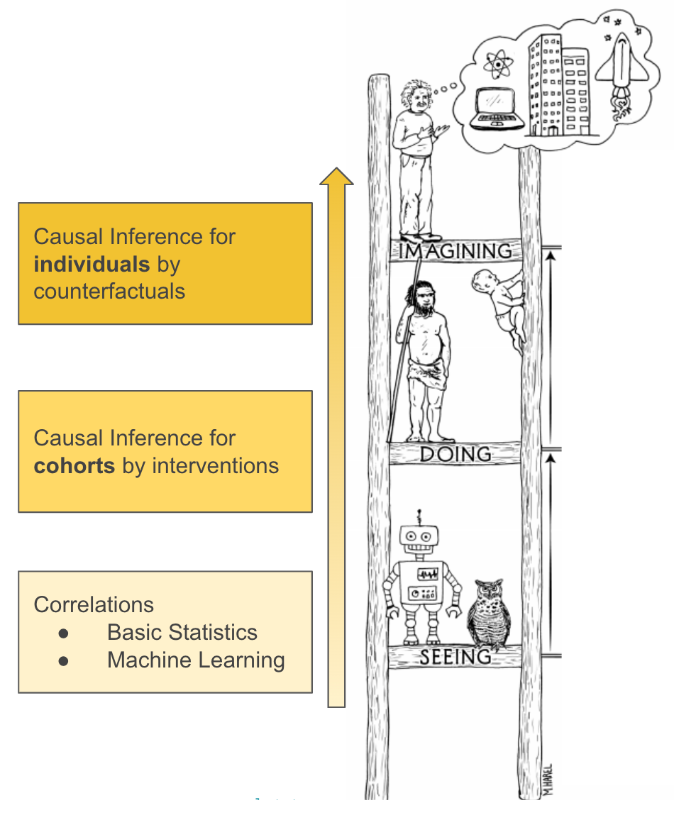
- Pearl’s Causal Hierarchy of seeing, doing and imagining (figure above)
- Observational data vs. Randomised Control Trials
- d-separation, common causes, colliders, mediators, instrumental variables
- Causal Graphs
- Structural Causal Models
- Assumptions: Ignorability, SUTVA, Consistency, Positivity
- “Do” Algebra — assessing impact on cohorts by intervention
- Counterfactuals — assessing impact on individuals by comparing real outcomes to potential ones
- The fundamental problem of causality
- Estimand, Estimator, Estimate, Identifiability — relating causal definitions to observable statistics (e.g, conditional probabilities)
- Causal Discovery — finding causal graphs with data (e.g, Markov Equivalence)
- Causal Machine Learning (e.g, Double Machine Learning)
For completeness it is useful to know that there are different streams of causality. Although there is a lot of overlap you may find that methods differ in naming convention due to development in different fields of research: Computer Science, Social Sciences, Health, Economics
Here I used definitions mostly from the Pearlian perspective (as developed in the field of computer science).
The Story Behind This Post
This narrative is a result of two study groups that I have conducted in a previous role to get myself and colleagues to learn about causality, which I felt missing in my skill set. If there is any interest I’m glad to write a post about the study group experience.
This intro was created as the one I felt that I needed when I started my journey in causality.
In the first iteration of this post I wrote and presented the limitations of spurious correlations and Simpson’s paradox. The main reason for this revision to focus on two paradoxes is that, whereas most causality intros focus on the limitations of correlations, I feel that understanding the concept of justification of confounders is important for all analysts and machine learning practitioners to be aware of.
On September 5th 2024 I have presented this content in a contributed talk at the Royal Statistical Society Annual Conference in Brighton, England (abstract link).

Unfortunately there is no recording but there are of previous talks of mine:
The slides are available at bit.ly/start-ask-why.
Start Asking Data Why | Causality Intro| Eyal Kazin was originally published in Towards Data Science on Medium, where people are continuing the conversation by highlighting and responding to this story.
from Datascience in Towards Data Science on Medium https://ift.tt/0dgrA9S
via IFTTT


