
What’s Inside a Neural Network?
Plotting surface of error in 3D using PyTorch🔥
In my senior year of undergrad, like many other students, I had to choose a topic for my bachelor’s thesis. My major was hydrometeorology, so I initially considered researching a problem related to climate modeling. Fortunately, my advisor, Dr. Gribanov, suggested exploring a completely new direction I knew nothing about at the time — applying Neural Networks to upscale terrestrial carbon fluxes. Back then, the word “neural” made me think of surgery, and “network” of transportation. However, he gave me one of the clearest and most intuitive explanations of neural networks I’ve ever heard. One of the highlights was his description of the optimization process.
Imagine a piece of blank paper like this:

Now I ask you to aggressively (it’s important) crumple it to a ball:

After straightening it back you’ll see something like an earth surface or some kind of a landscape with its peaks and depressions:

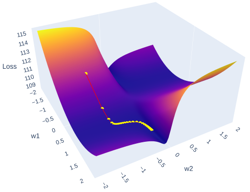
Now, if we introduce three dimensions — weight 1 , weight 2, and mean squared error (MSE) instead of latitude, longitude and elevation — we can think of this image as representing the error surface of a neural network. The goal of optimization is to find the lowest point on this surface, which corresponds to the minimum error. As you can see from the image there is a multitude of local minima and maxima, that’s why it’s always a challenging task.
So in this article, we will create such a surface in 3D and use the plotly Python library to interactively illustrate it, along with the steps of Stochastic Gradient Descent (SGD).
As always the code of this article you can find on my GitHub.
Data
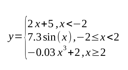
First and foremost, we need synthetic data to work with. The data should exhibit some non-linear dependency. Let’s define it like this:
In python it will have the following shape:
np.random.seed(42)
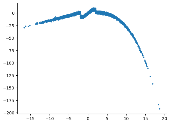
X = np.random.normal(1, 4.5, 10000)
y = np.piecewise(X, [X < -2,(X >= -2) & (X < 2), X >= 2], [lambda X: 2*X + 5, lambda X: 7.3*np.sin(X), lambda X: -0.03*X**3 + 2]) + np.random.normal(0, 1, X.shape)
After visualization:
Neural Net
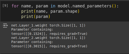
Since we are visualizing a 3D space, our neural network will only have 2 weights. This means the ANN will consist of a single hidden neuron. Implementing this in PyTorch is quite intuitive:
class ANN(nn.Module):
    def __init__(self, input_size, N, output_size):
        super().__init__()
        self.net = nn.Sequential()
        self.net.add_module(name='Layer_1', module=nn.Linear(input_size, N, bias=False))
        self.net.add_module(name='Tanh',module=nn.Tanh())
        self.net.add_module(name='Layer_2',module=nn.Linear(N, output_size, bias=False))


    def forward(self, x):
        return self.net(x)
Important! Don’t forget to turn off the biases in your layers, otherwise you’ll end up having x2 more parameters.
Changing weights
To build the error surface, we first need to create a grid of possible values for W1 and W2. Then, for each weight combination, we will update the parameters of the network and calculate the error:
W1, W2 = np.arange(-2, 2, 0.05), np.arange(-2, 2, 0.05)
LOSS = np.zeros((len(W1), len(W2)))
for i, w1 in enumerate(W1):
    model.net._modules['Layer_1'].weight.data = torch.tensor([[w1]], dtype=torch.float32)

    for j, w2 in enumerate(W2):
        model.net._modules['Layer_2'].weight.data = torch.tensor([[w2]], dtype=torch.float32)

        model.eval()
        total_loss = 0
        with torch.no_grad():
            for x, y in test_loader:
                preds = model(x.reshape(-1, 1))
                total_loss += loss(preds, y).item()

        LOSS[i, j] = total_loss / len(test_loader)
It may take some time. If you make the resolution of this grid too coarse (i.e., the step size between possible weight values), you might miss local minima and maxima. Remember how the learning rate is often schedule to decrease over time? When we do this, the absolute change in weight values can be as small as 1e-3 or less. A grid with a 0.5 step simply won’t capture these fine details of the error surface!
Training the model
At this point, we don’t care at all about the quality of the trained model. However, we do want to pay attention to the learning rate, so let’s keep it between 1e-1 and 1e-2. We’ll simply collect the weight values and errors during the training process and store them in separate lists:
model = ANN(1,1,1)
epochs = 25
lr = 1e-2

optimizer = optim.SGD(model.parameters(),lr =lr)

model.net._modules['Layer_1'].weight.data = torch.tensor([[-1]], dtype=torch.float32)
model.net._modules['Layer_2'].weight.data = torch.tensor([[-1]], dtype=torch.float32)

errors, weights_1, weights_2 = [], [], []

model.eval()
with torch.no_grad():
    total_loss = 0
    for x, y in test_loader:
        preds = model(x.reshape(-1,1))
        error = loss(preds, y)
        total_loss += error.item()
weights_1.append(model.net._modules['Layer_1'].weight.data.item())
weights_2.append(model.net._modules['Layer_2'].weight.data.item())
errors.append(total_loss / len(test_loader))

for epoch in tqdm(range(epochs)):
    model.train()

    for x, y in train_loader:
        pred = model(x.reshape(-1,1))
        error = loss(pred, y)
        optimizer.zero_grad()
        error.backward()
        optimizer.step()

    model.eval()
    test_preds, true = [], []
    with torch.no_grad():
        total_loss = 0
        for x, y in test_loader:
            preds = model(x.reshape(-1,1))
            error = loss(preds, y)
            test_preds.append(preds)
            true.append(y)

            total_loss += error.item()
    weights_1.append(model.net._modules['Layer_1'].weight.data.item())
    weights_2.append(model.net._modules['Layer_2'].weight.data.item())
    errors.append(total_loss / len(test_loader))
Visualization
Finally, we can visualize the data we have collected using plotly. The plot will have two scenes: surface and SGD trajectory. One of the ways to do the first part is to create a figure with a plotly surface. After that we will style it a little by updating a layout.
The second part is as simple as it is — just use Scatter3d function and specify all three axes.
import plotly.graph_objects as go
import plotly.io as pio

plotly_template = pio.templates["plotly_dark"]
fig = go.Figure(data=[go.Surface(z=LOSS, x=W1, y=W2)])

fig.update_layout(
    title='Loss Surface',
    scene=dict(
        xaxis_title='w1',
        yaxis_title='w2',
        zaxis_title='Loss',
        aspectmode='manual',
        aspectratio=dict(x=1, y=1, z=0.5),
        xaxis=dict(showgrid=False),
        yaxis=dict(showgrid=False),
        zaxis=dict(showgrid=False),
    ),
    width=800,
    height=800
)

fig.add_trace(go.Scatter3d(x=weights_2, y=weights_1, z=errors,
                               mode='lines+markers',
                              line=dict(color='red', width=2),
                              marker=dict(size=4, color='yellow') ))
fig.show()
Running it in Google Colab or locally in Jupyter Notebook will allow you to investigate the error surface more closely. Honestly, I spent a buch of time just looking at this figure:)
I’d love to see you surfaces, so please feel free to share it in comments. I strongly believe that the more imperfect the surface is the more interesting it is to investigate it!
===========================================
All my publications on Medium are free and open-access, that’s why I’d really appreciate if you followed me here!
P.s. I’m extremely passionate about (Geo)Data Science, ML/AI and Climate Change. So if you want to work together on some project pls contact me in LinkedIn and check out my website!
🛰️Follow for more🛰️
What’s Inside a Neural Network? was originally published in Towards Data Science on Medium, where people are continuing the conversation by highlighting and responding to this story.
from Datascience in Towards Data Science on Medium https://ift.tt/hoCK4RI
via IFTTT


