
K Nearest Neighbor Regressor, Explained: A Visual Guide with Code Examples
REGRESSION ALGORITHM
Finding the neighbors FAST with KD Trees and Ball Trees
K Nearest Neighbor Classifier, Explained: A Visual Guide with Code Examples for Beginners
Building on our exploration of the Nearest Neighbor Classifier, let’s turn to its sibling in the regression world. The Nearest Neighbor Regressor applies the same intuitive concept to predicting continuous values. But as our datasets get bigger, finding these neighbors efficiently becomes a real pain. That’s where KD Trees and Ball Trees come in.
It’s super frustrating that there’s no clear guide out there that really explains what’s going on with these algorithms. Sure, there are some 2D visualizations, but they often don’t make it clear how the trees work in multidimensional setting.
Here, we will explain what’s actually going on in these algorithms without using the oversimplified 2D representation. We’ll be focusing on the construction of the trees itself and see which computation (and numbers) actually matters.

Definition
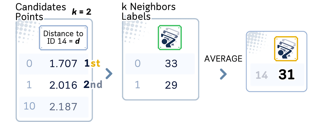
The Nearest Neighbor Regressor is a straightforward predictive model that estimates values by averaging the outcomes of nearby data points. This method builds on the idea that similar inputs likely yield similar outputs.
📊 Dataset Used
To illustrate our concepts, we’ll use our usual dataset. This dataset helps predict the number of golfers visiting on any given day. It includes factors such as weather outlook, temperature, humidity, and wind conditions. Our goal is to estimate the daily golfer turnout based on these variables.
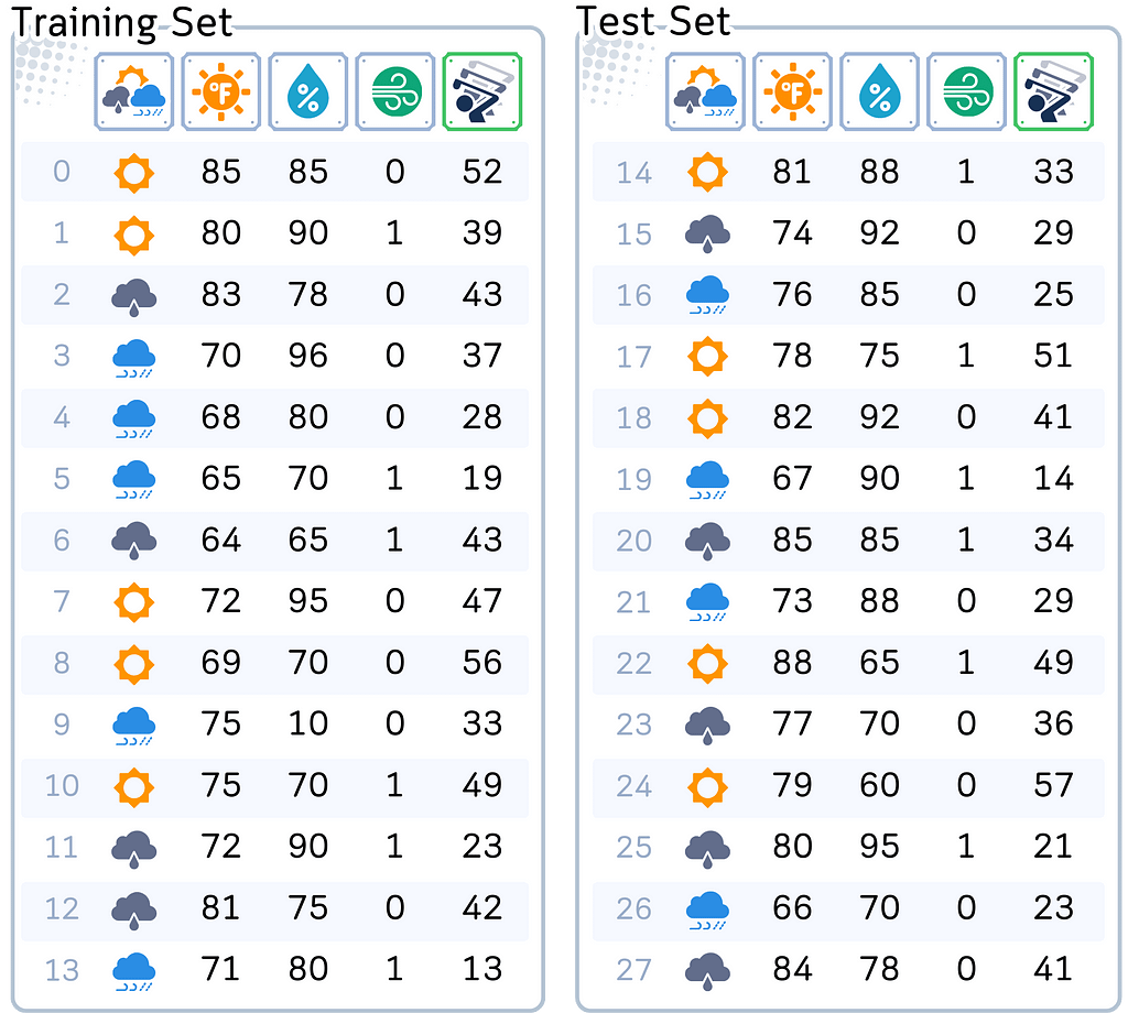
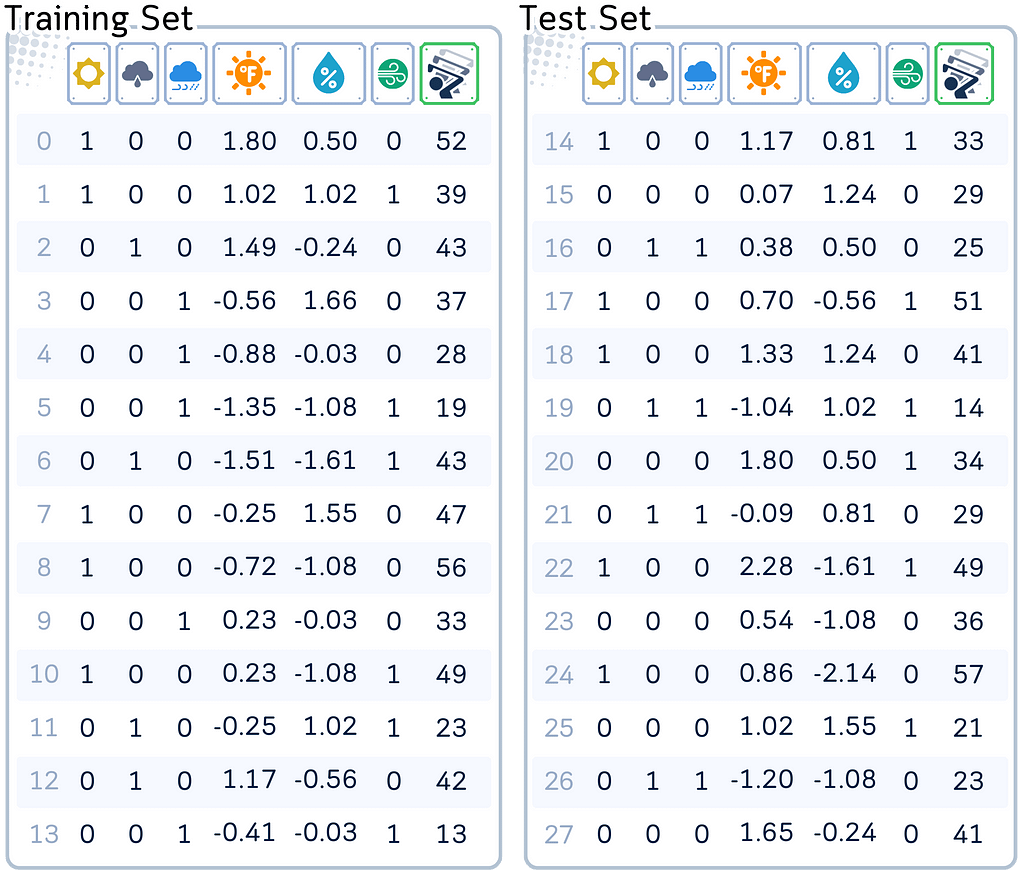
To use Nearest Neighbor Regression effectively, we need to preprocess our data. This involves converting categorical variables into numerical format and scaling numerical features.
# Import libraries
import pandas as pd
import numpy as np
from sklearn.model_selection import train_test_split
from sklearn.metrics import root_mean_squared_error
from sklearn.neighbors import KNeighborsRegressor
from sklearn.preprocessing import StandardScaler
from sklearn.compose import ColumnTransformer

# Create dataset
dataset_dict = {
    'Outlook': ['sunny', 'sunny', 'overcast', 'rain', 'rain', 'rain', 'overcast', 'sunny', 'sunny', 'rain', 'sunny', 'overcast', 'overcast', 'rain', 'sunny', 'overcast', 'rain', 'sunny', 'sunny', 'rain', 'overcast', 'rain', 'sunny', 'overcast', 'sunny', 'overcast', 'rain', 'overcast'],
    'Temperature': [85.0, 80.0, 83.0, 70.0, 68.0, 65.0, 64.0, 72.0, 69.0, 75.0, 75.0, 72.0, 81.0, 71.0, 81.0, 74.0, 76.0, 78.0, 82.0, 67.0, 85.0, 73.0, 88.0, 77.0, 79.0, 80.0, 66.0, 84.0],
    'Humidity': [85.0, 90.0, 78.0, 96.0, 80.0, 70.0, 65.0, 95.0, 70.0, 80.0, 70.0, 90.0, 75.0, 80.0, 88.0, 92.0, 85.0, 75.0, 92.0, 90.0, 85.0, 88.0, 65.0, 70.0, 60.0, 95.0, 70.0, 78.0],
    'Wind': [False, True, False, False, False, True, True, False, False, False, True, True, False, True, True, False, False, True, False, True, True, False, True, False, False, True, False, False],
    'Num_Players': [52, 39, 43, 37, 28, 19, 43, 47, 56, 33, 49, 23, 42, 13, 33, 29, 25, 51, 41, 14, 34, 29, 49, 36, 57, 21, 23, 41]
}

df = pd.DataFrame(dataset_dict)

# One-hot encode 'Outlook' column
df = pd.get_dummies(df, columns=['Outlook'])

# Convert 'Wind' column to binary
df['Wind'] = df['Wind'].astype(int)

# Split data into features and target, then into training and test sets
X, y = df.drop(columns='Num_Players'), df['Num_Players']
X_train, X_test, y_train, y_test = train_test_split(X, y, train_size=0.5, shuffle=False)

# Identify numerical columns
numerical_columns = ['Temperature', 'Humidity']

# Create a ColumnTransformer to scale only numerical columns
ct = ColumnTransformer([
    ('scaler', StandardScaler(), numerical_columns)
], remainder='passthrough')

# Fit the ColumnTransformer on the training data and transform both training and test data
X_train_transformed = ct.fit_transform(X_train)
X_test_transformed = ct.transform(X_test)

# Convert the transformed data back to DataFrames
feature_names = numerical_columns + [col for col in X_train.columns if col not in numerical_columns]
X_train_scaled = pd.DataFrame(X_train_transformed, columns=feature_names, index=X_train.index)
X_test_scaled = pd.DataFrame(X_test_transformed, columns=feature_names, index=X_test.index)
Main Mechanism
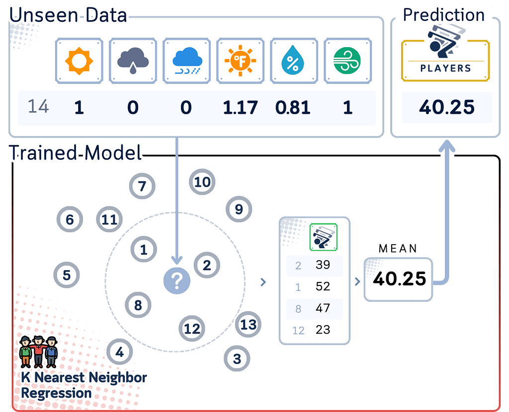
The Nearest Neighbor Regressor works similarly to its classifier counterpart, but instead of voting on a class, it averages the target values. Here’s the basic process:
- Calculate the distance between the new data point and all points in the training set.
- Select the K nearest neighbors based on these distances.
- Calculate the average of the target values of these K neighbors.
- Assign this average as the predicted value for the new data point.
The approach above, using all data points to find neighbors, is known as the Brute Force method. It’s straightforward but can be slow for large datasets.
Here, we’ll explore two more efficient algorithms for finding nearest neighbors:
KD Tree for KNN Regression
KD Tree (K-Dimensional Tree) is a binary tree structure used for organizing points in a k-dimensional space. It’s particularly useful for tasks like nearest neighbor searches and range searches in multidimensional data.
Training Steps:
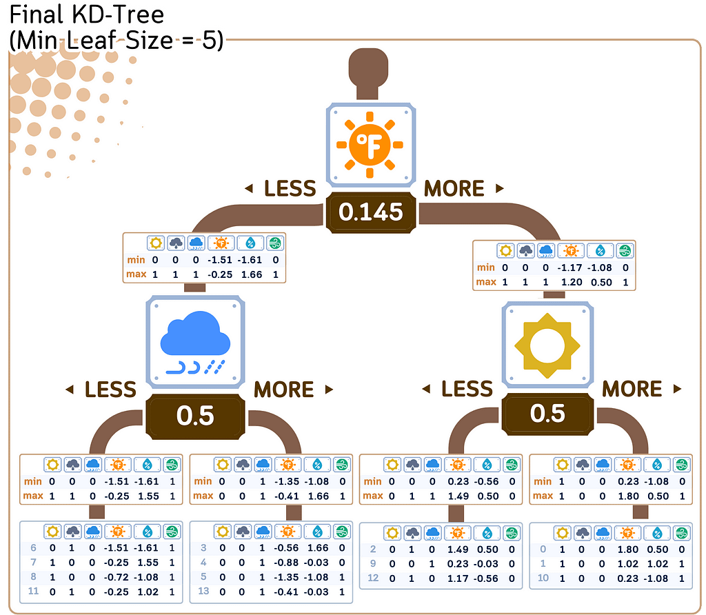
1. Build the KD Tree:
a. Start with a root node that contains all the points.
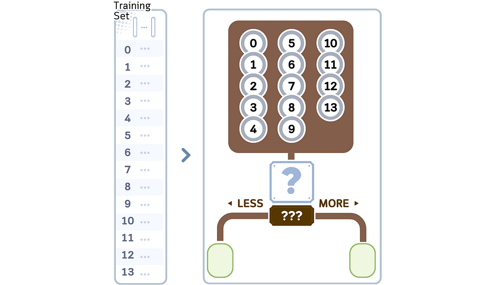
b. Choose a feature to split on. Any random feature should be ok actually, but another good way to choose this is by looking which feature has median value closest to the midpoint between max and min value.
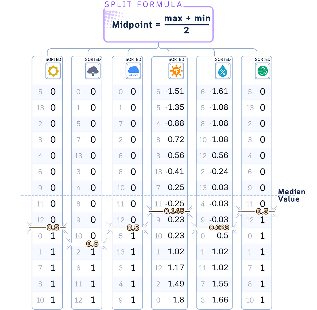
c. Split the tree in the chosen feature and midpoint.
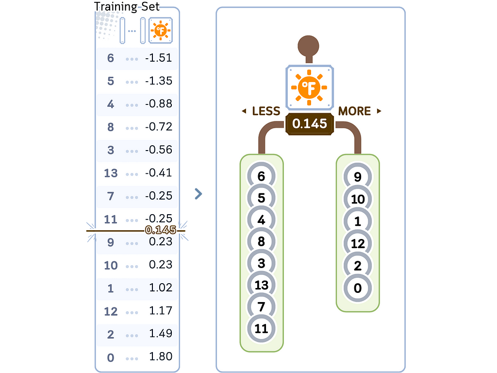
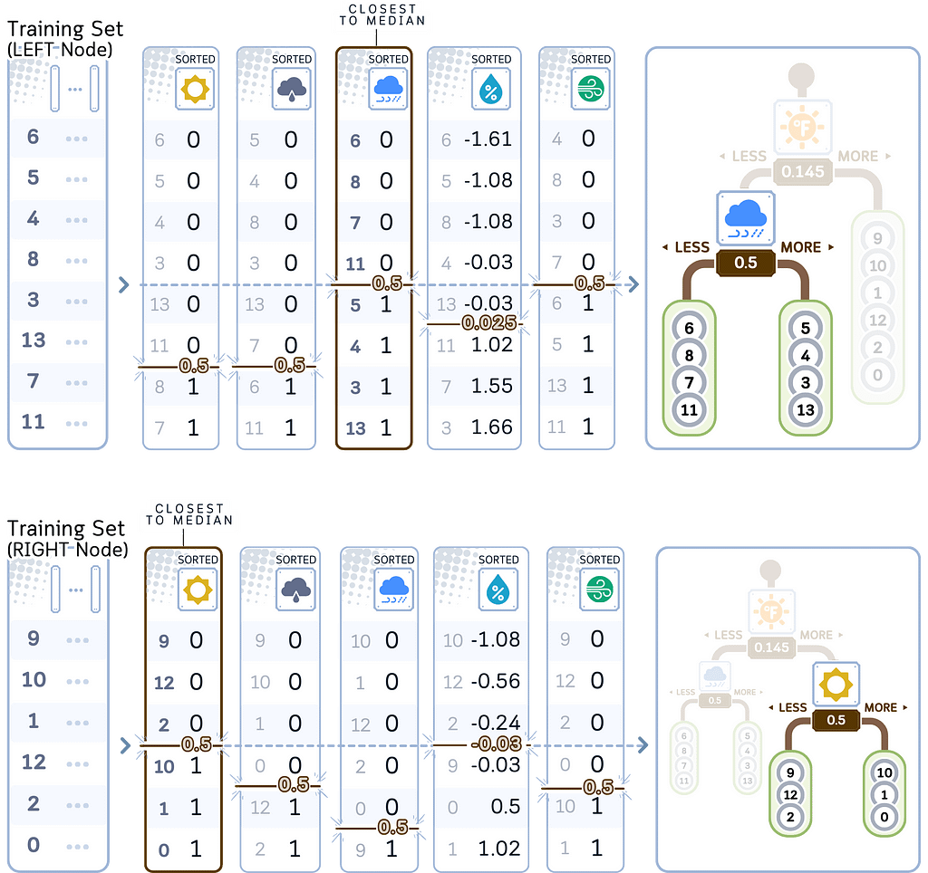
d. Recursively, do step a-c until the stopping criterion, usually minimal leaf size (see “min samples leaf” here)
2. Store the target values:
Along with each point in the KD Tree, store its corresponding target value. The minimum and maximum value for each node are also stored.
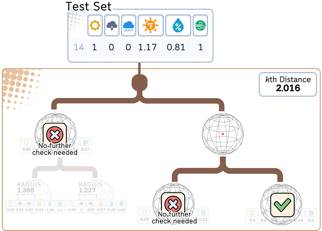
Regression/Prediction Steps:
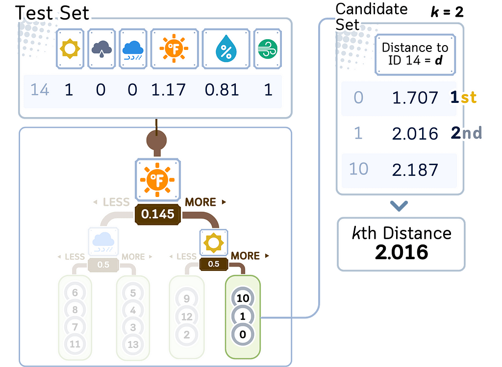
1. Traverse the KD Tree:
a. Start at the root node.
b. Compare the query point (test point) with the splitting dimension and value at each node.
c. Recursively traverse left or right based on this comparison.
d. When reaching a leaf node, add its points to the candidate set.
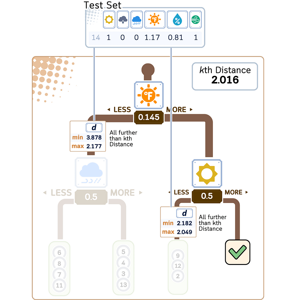
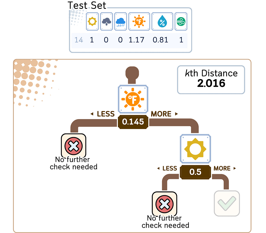
2. Refine the search:
a. Backtrack through the tree, checking if there could be closer points in other branches.
b. Use distance calculations to the maximum and minimum of the unexplored branches to determine if exploring is necessary.
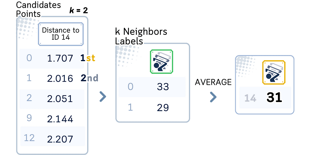
3. Find K nearest neighbors:
a. Among the candidate points found, select the K points closest to the query point.
4. Perform regression:
a. Calculate the average of the target values of the K nearest neighbors.
b. This average is the predicted value for the query point.
By using a KD Tree, the average time complexity for finding nearest neighbors can be reduced from O(n) in the brute force method to O(log n) in many cases, where n is the number of points in the dataset. This makes KNN Regression much more efficient for large datasets.
Ball Tree for KNN Regression
Ball Tree is another space-partitioning data structure that organizes points in a series of nested hyperspheres. It’s particularly effective for high-dimensional data where KD Trees may become less efficient.
Training Steps:
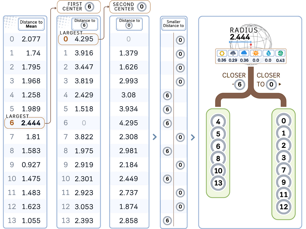
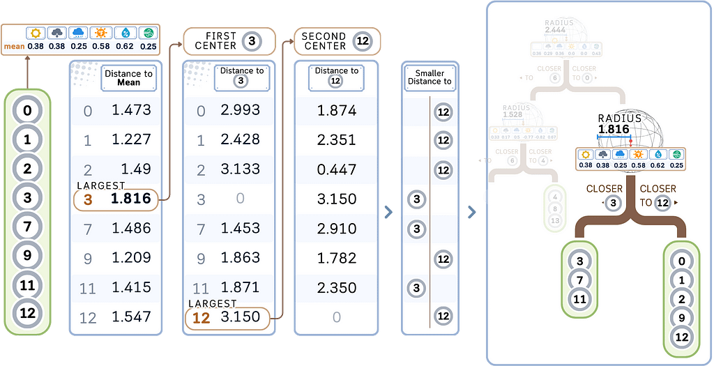
1. Build the Ball Tree:
a. Calculate the centroid of all points in the node (the mean). This becomes the pivot point.
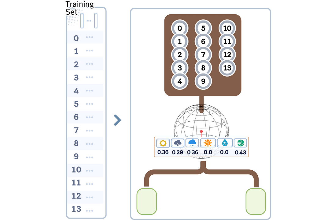
b. Make the first branch:
- Finding the first center: Choose the furthest point from the pivot point as the first center with its distance as the radius.
- Finding the second center: From the first center, select the furthest point as the second center.
- Partitioning: Divide the remaining points into two child nodes based on which center they are closer to.
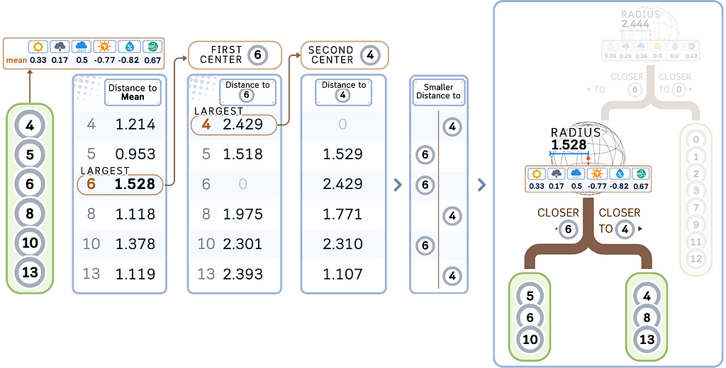
d. Recursively apply steps a-b to each child node until a stopping criterion is met, usually minimal leaf size (see “min samples leaf” here).
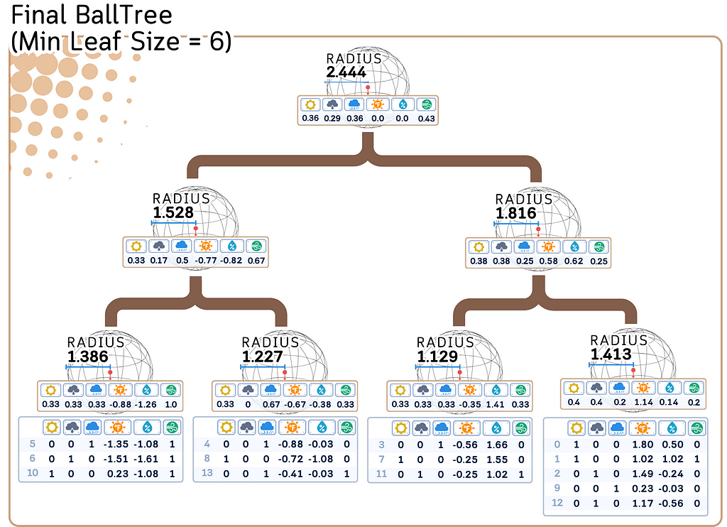
2. Store the target values:
Along with each point in the Ball Tree, store its corresponding target value. The radius and centroid for each node are also stored.
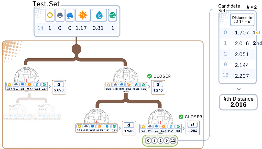
Regression/Prediction Steps:
1. Traverse the Ball Tree:
a. Start at the root node.
b. At each node, calculate the distance between the unseen data and the center of each child hypersphere.
c. Traverse into the closest hypersphere first.
d. When reaching a leaf node, add its points to the candidate set.
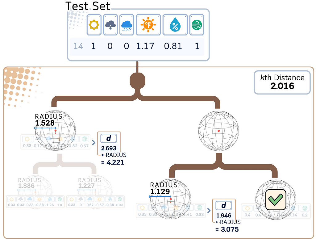
2. Refine the search:
a. Determine if other branches need to be explored.
b. If the distance to a hypersphere plus its radius is greater than the current Kth nearest distance, that branch can be safely ignored.
3. Find K nearest neighbors:
a. Among the candidate points found, select the K points closest to the query point.
4. Perform regression:
a. Calculate the average of the target values of the K nearest neighbors.
b. This average is the predicted value for the query point.
Ball Trees can be more efficient than KD Trees for high-dimensional data or when the dimensionality is greater than the log of the number of samples. They maintain good performance even when the number of dimensions increases, making them suitable for a wide range of datasets.
The time complexity for querying in a Ball Tree is O(log n) on average, similar to KD Trees, but Ball Trees often perform better in higher dimensions where KD Trees may degrade to linear time complexity.
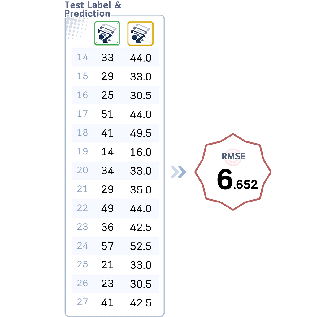
Evaluation Step (Brute Force, KD Tree, Ball Tree)
Regardless of the algorithm we choose, all of them give the same following result:
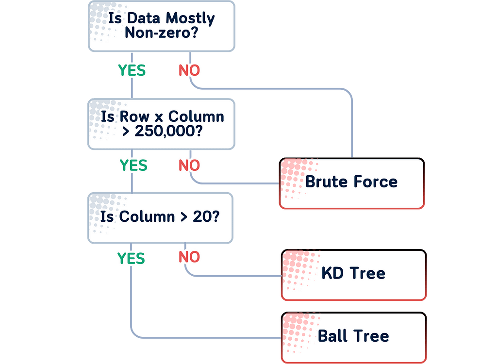
Which Algorithm to Choose?
You can follow this simple rule for choosing the best one:
- For small datasets (< 1000 samples), ‘brute’ might be fast enough and guarantees finding the exact nearest neighbors.
- For larger datasets with few features (< 20), ‘kd_tree’ is usually the fastest.
- For larger datasets with many features, ‘ball_tree’ often performs best.
The ‘auto’ option in scikit-learn typically follow the following chart:
Key Parameters
While KNN regression has many other parameter, other than the algorithm we just discussed (brute force, kd tree, ball tree), you mainly need to consider
- Number of Neighbors (K).
- Smaller K: More sensitive to local patterns, but may lead to overfitting.
- Larger K: Smoother predictions, but might miss important local variations.
Unlike classification, even numbers are fine in regression as we’re averaging values. - Leaf Size
This is the stopping condition for building kd tree or ball tree. Generally, It affects the speed of construction and query, as well as the memory required to store the tree.
Pros & Cons
Pros:
- Simplicity and Versatility: Easy to understand and implement; can be used for both classification and regression tasks.
- No Assumptions: Doesn’t assume anything about the data distribution, making it suitable for complex datasets.
- No Training Phase: Can quickly incorporate new data without retraining.
- Interpretability: Predictions can be explained by examining nearest neighbors.
Cons:
- Computational Complexity: Prediction time can be slow, especially with large datasets, though optimized algorithms (KD-Tree, Ball Tree) can help for lower dimensions.
- Curse of Dimensionality: Performance degrades in high-dimensional spaces, affecting both accuracy and efficiency.
- Memory Intensive: Requires storing all training data.
- Sensitive to Feature Scaling and Irrelevant Features: Can be biased by features on larger scales or those unimportant to the prediction.
Final Remarks
The K-Nearest Neighbors (KNN) regressor is a basic yet powerful tool in machine learning. Its straightforward approach makes it great for beginners, and its flexibility ensures it’s useful for experts too.
As you learn more about data analysis, use KNN to understand the basics of regression before exploring more advanced methods. By mastering KNN and how to compute the nearest neighbors, you’ll build a strong foundation for tackling more complex challenges in data analysis.
🌟 k Nearest Neighbor Regressor Code Summarized
# Import libraries
import pandas as pd
import numpy as np
from sklearn.model_selection import train_test_split
from sklearn.metrics import root_mean_squared_error
from sklearn.neighbors import KNeighborsRegressor
from sklearn.preprocessing import StandardScaler
from sklearn.compose import ColumnTransformer

# Create dataset
dataset_dict = {
    'Outlook': ['sunny', 'sunny', 'overcast', 'rain', 'rain', 'rain', 'overcast', 'sunny', 'sunny', 'rain', 'sunny', 'overcast', 'overcast', 'rain', 'sunny', 'overcast', 'rain', 'sunny', 'sunny', 'rain', 'overcast', 'rain', 'sunny', 'overcast', 'sunny', 'overcast', 'rain', 'overcast'],
    'Temperature': [85.0, 80.0, 83.0, 70.0, 68.0, 65.0, 64.0, 72.0, 69.0, 75.0, 75.0, 72.0, 81.0, 71.0, 81.0, 74.0, 76.0, 78.0, 82.0, 67.0, 85.0, 73.0, 88.0, 77.0, 79.0, 80.0, 66.0, 84.0],
    'Humidity': [85.0, 90.0, 78.0, 96.0, 80.0, 70.0, 65.0, 95.0, 70.0, 80.0, 70.0, 90.0, 75.0, 80.0, 88.0, 92.0, 85.0, 75.0, 92.0, 90.0, 85.0, 88.0, 65.0, 70.0, 60.0, 95.0, 70.0, 78.0],
    'Wind': [False, True, False, False, False, True, True, False, False, False, True, True, False, True, True, False, False, True, False, True, True, False, True, False, False, True, False, False],
    'Num_Players': [52, 39, 43, 37, 28, 19, 43, 47, 56, 33, 49, 23, 42, 13, 33, 29, 25, 51, 41, 14, 34, 29, 49, 36, 57, 21, 23, 41]
}

df = pd.DataFrame(dataset_dict)

# One-hot encode 'Outlook' column
df = pd.get_dummies(df, columns=['Outlook'])

# Convert 'Wind' column to binary
df['Wind'] = df['Wind'].astype(int)

# Split data into features and target, then into training and test sets
X, y = df.drop(columns='Num_Players'), df['Num_Players']
X_train, X_test, y_train, y_test = train_test_split(X, y, train_size=0.5, shuffle=False)

# Identify numerical columns
numerical_columns = ['Temperature', 'Humidity']

# Create a ColumnTransformer to scale only numerical columns
ct = ColumnTransformer([
    ('scaler', StandardScaler(), numerical_columns)
], remainder='passthrough')

# Fit the ColumnTransformer on the training data and transform both training and test data
X_train_transformed = ct.fit_transform(X_train)
X_test_transformed = ct.transform(X_test)

# Convert the transformed data back to DataFrames
feature_names = numerical_columns + [col for col in X_train.columns if col not in numerical_columns]
X_train_scaled = pd.DataFrame(X_train_transformed, columns=feature_names, index=X_train.index)
X_test_scaled = pd.DataFrame(X_test_transformed, columns=feature_names, index=X_test.index)

# Initialize and train KNN Regressor
knn = KNeighborsRegressor(n_neighbors=5,
                          algorithm='kd_tree', #'ball_tree', 'brute'
                          leaf_size=5) #default is 30
knn.fit(X_train_scaled, y_train)

# Make predictions
y_pred = knn.predict(X_test_scaled)

# Calculate and print RMSE
rmse = root_mean_squared_error(y_test, y_pred)
print(f"RMSE: {rmse:.4f}")
Further Reading
For a detailed explanation of the KNeighborsRegressor, KDTree, BallTree, and its implementation in scikit-learn, readers can refer to their official documentation. It provides comprehensive information on their usage and parameters.
Technical Environment
This article uses Python 3.7 and scikit-learn 1.5. While the concepts discussed are generally applicable, specific code implementations may vary slightly with different versions
About the Illustrations
Unless otherwise noted, all images are created by the author, incorporating licensed design elements from Canva Pro.
K Nearest Neighbor Regressor, Explained: A Visual Guide with Code Examples was originally published in Towards Data Science on Medium, where people are continuing the conversation by highlighting and responding to this story.
from Datascience in Towards Data Science on Medium https://ift.tt/PS0Cw4T
via IFTTT


