Lessons in Decision Making from the Monty Hall Problem
A journey into three intuitions: Common, Bayesian and Causal

The Monty Hall Problem is a well-known brain teaser from which we can learn important lessons in decision making that are useful in general and in particular for data scientists.
If you are not familiar with this problem, prepare to be perplexed 🤯. If you are, I hope to shine light on aspects that you might not have considered 💡.
I introduce the problem and solve with three types of intuitions:
- Common — The heart of this post focuses on applying our common sense to solve this problem. We’ll explore why it fails us 😕 and what we can do to intuitively overcome this to make the solution crystal clear 🤓. We’ll do this by using visuals 🎨 , qualitative arguments and some basic probabilities (not too deep, I promise).
- Bayesian — We will briefly discuss the importance of belief propagation.
- Causal — We will use a Graph Model to visualise conditions required to use the Monty Hall problem in real world settings.
🚨Spoiler alert 🚨 I haven’t been convinced that there are any, but the thought process is very useful.
I summarise by discussing lessons learnt for better data decision making.
In regards to the Bayesian and Causal intuitions, these will be presented in a gentle form. For the mathematically inclined ⚔️ I also provide supplementary sections with short deep dives into each approach after the summary. (Note: These are not required to appreciate the main points of the article.)
By examining different aspects of this puzzle in probability 🧩 you will hopefully be able to improve your data decision making ⚖️.

First, some history. Let’s Make a Deal is a USA television game show that originated in 1963. As its premise, audience participants were considered traders making deals with the host, Monty Hall 🎩.
At the heart of the matter is an apparently simple scenario:
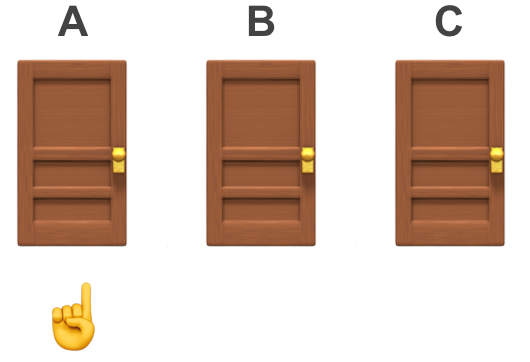
A trader is posed with the question of choosing one of three doors for the opportunity to win a luxurious prize, e.g, a car 🚗. Behind the other two were goats 🐐.

The trader chooses one of the doors. Let’s call this (without loss of generalisability) door A and mark it with a ☝️.
Keeping the chosen door ☝️ closed️, the host reveals one of the remaining doors showing a goat 🐐 (let’s call this door C).
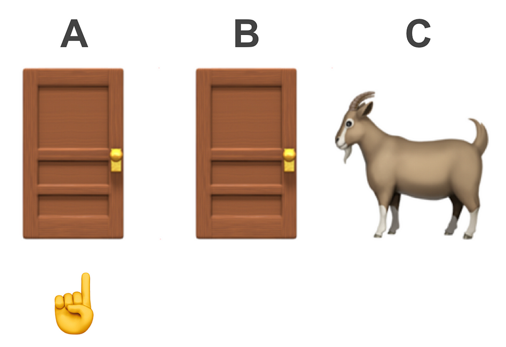
The host then asks the trader if they would like to stick with their first choice ☝️ or switch to the other remaining one (which we’ll call door B).
If the trader guesses correct they win the prize 🚗. If not they’ll be shown another goat 🐐 (also referred to as a zonk).

Should the trader stick with their original choice of door A or switch to B?
Before reading further, give it a go. What would you do?
Most people are likely to have a gut intuition that “it doesn’t matter” arguing that in the first instance each door had a ⅓ chance of hiding the prize, and that after the host intervention 🎩, when only two doors remain closed, the winning of the prize is 50:50.
There are various ways of explaining why the coin toss intuition is incorrect. Most of these involve maths equations, or simulations. Whereas we will address these later, we’ll attempt to solve by applying Occam’s razor:
A principle that states that simpler explanations are preferable to more complex ones — William of Ockham (1287–1347)
To do this it is instructive to slightly redefine the problem to a large N doors instead of the original three.
The Large N-Door Problem
Similar to before: you have to choose one of many doors. For illustration let’s say N=100. Behind one of the doors there is the prize 🚗 and behind 99 (N-1) of the rest are goats 🐐.

You choose one door 👇 and the host 🎩 reveals 98 (N-2) of the other doors that have goats 🐐 leaving yours 👇 and one more closed 🚪.
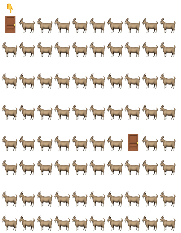
Should you stick with your original choice or make the switch?
I think you’ll agree with me that the remaining door, not chosen by you, is much more likely to conceal the prize … so you should definitely make the switch!
It’s illustrative to compare both scenarios discussed so far. In the next figure we compare the post host intervention for the N=3 setup (top panel) and that of N=100 (bottom):

In both cases we see two shut doors, one of which we’ve chosen. The main difference between these scenarios is that in the first we see one goat and in the second there are more than the eye would care to see (unless you shepherd for a living).
Why do most people consider the first case as a “50:50” toss up and in the second it’s obvious to make the switch?
We’ll soon address this question of why. First let’s put probabilities of success behind the different scenarios.
What’s The Frequency, Kenneth?
So far we learnt from the N=100 scenario that switching doors is obviously beneficial. Inferring for the N=3 may be a leap of faith for most. Using some basic probability arguments here we’ll quantify why it is favourable to make the switch for any number door scenario N.
We start with the standard Monty Hall problem (N=3). When it starts the probability of the prize being behind each of the doors A, B and C is p=⅓. To be explicit let’s define the Y parameter to be the door with the prize 🚗, i.e, p(Y=A)= p(Y=B)=p(Y=C)=⅓.
The trick to solving this problem is that once the trader’s door A has been chosen ☝️, we should pay close attention to the set of the other doors {B,C}, which has the probability of p(Y∈{B,C})=p(Y=B)+p(Y=C)=⅔. This visual may help make sense of this:
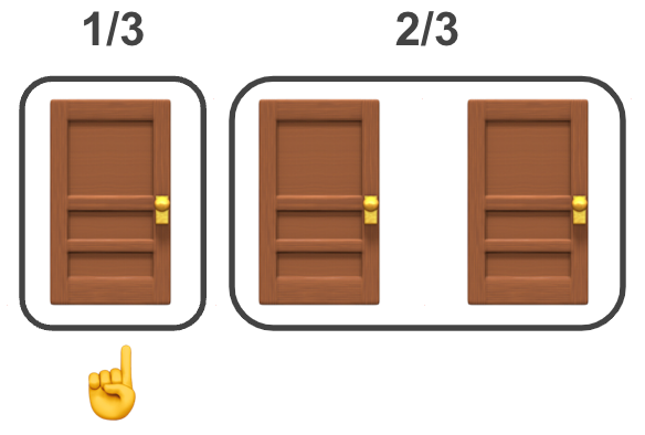
By being attentive to the {B,C} the rest should follow. When the goat 🐐 is revealed
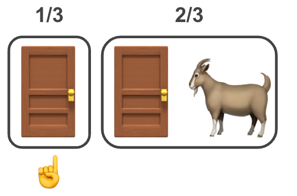
it is apparent that the probabilities post intervention change. Note that for ease of reading I’ll drop the Y notation, where p(Y=A) will read p(A) and p(Y∈{B,C}) will read p({B,C}). Also for completeness the full terms after the intervention should be even longer due to it being conditional, e.g, p(Y=A|Z=C), p(Y∈{B,C}|Z=C), where Z is a parameter representing the choice of the host 🎩. (In the Bayesian supplement section below I use proper notation without this shortening.)
- p(A) remains ⅓
- p({B,C})=p(B)+p(C) remains ⅔,
- p(C)=0; we just learnt that the goat 🐐 is behind door C, not the prize.
- p(B)= p({B,C})-p(C) = ⅔
For anyone with the information provided by the host (meaning the trader and the audience) this means that it isn’t a toss of a fair coin! For them the fact that p(C) became zero does not “raise all other boats” (probabilities of doors A and B), but rather p(A) remains the same and p(B) gets doubled.
The bottom line is that the trader should consider p(A) = ⅓ and p(B)=⅔, hence by switching they are doubling the odds at winning!
Let’s generalise to N (to make the visual simpler we’ll use N=100 again as an analogy).
When we start all doors have odds of winning the prize p=1/N. After the trader chooses one door which we’ll call D₁, meaning p(Y=D₁)=1/N, we should now pay attention to the remaining set of doors {D₂, …, Dₙ} will have a chance of p(Y∈{D₂, …, Dₙ})=(N-1)/N.

When the host reveals (N-2) doors {D₃, …, Dₙ} with goats (back to short notation):
- p(D₁) remains 1/N
- p({D₂, …, Dₙ})=p(D₂)+p(D₃)+… + p(Dₙ) remains (N-1)/N
- p(D₃)=p(D₄)= …=p(Dₙ₋₁) =p(Dₙ) = 0; we just learnt that they have goats, not the prize.
- p(D₂)=p({D₂, …, Dₙ}) — p(D₃) — … — p(Dₙ)=(N-1)/N
The trader should now consider two door values p(D₁)=1/N and p(D₂)=(N-1)/N.
Hence the odds of winning improved by a factor of N-1! In the case of N=100, this means by an odds ratio of 99! (i.e, 99% likely to win a prize when switching vs. 1% if not).
The improvement of odds ratios in all scenarios between N=3 to 100 may be seen in the following graph. The thin line is the probability of winning by choosing any door prior to the intervention p(Y)=1/N. Note that it also represents the chance of winning after the intervention, if they decide to stick to their guns and not switch p(Y=D₁|Z={D₃…Dₙ}). (Here I reintroduce the more rigorous conditional form mentioned earlier.) The thick line is the probability of winning the prize after the intervention if the door is switched p(Y=D₂|Z={D₃…Dₙ})=(N-1)/N:
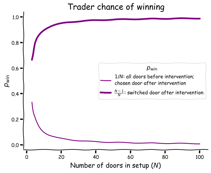
Perhaps the most interesting aspect of this graph (albeit also by definition) is that the N=3 case has the highest probability before the host intervention 🎩, but the lowest probability after and vice versa for N=100.
Another interesting feature is the quick climb in the probability of winning for the switchers:
- N=3: p=67%
- N=4: p=75%
- N=5=80%
The switchers curve gradually reaches an asymptote approaching at 100% whereas at N=99 it is 98.99% and at N=100 is equal to 99%.
This starts to address an interesting question:
Why Is Switching Obvious For Large N But Not N=3?
The answer is the fact that this puzzle is slightly ambiguous. Only the highly attentive realise that by revealing the goat (and never the prize!) the host is actually conveying a lot of information that should be incorporated into one’s calculation. Later we discuss the difference of doing this calculation in one’s mind based on intuition and slowing down by putting pen to paper or coding up the problem.
How much information is conveyed by the host by intervening?
A hand wavy explanation 👋 👋 is that this information may be visualised as the gap between the lines in the graph above. For N=3 we saw that the odds of winning doubled (nothing to sneeze at!), but that doesn’t register as strongly to our common sense intuition as the 99 factor as in the N=100.
I have also considered describing stronger arguments from Information Theory that provide useful vocabulary to express communication of information. However, I feel that this fascinating field deserves a post of its own.
To summarise this section, we use basic probability arguments to quantify the probabilities of winning the prize showing the benefit of switching for all N door scenarios. For those interested in more formal solutions ⚔️ using Bayesian and Causality on the bottom I provide supplement sections.
In the next three final sections we’ll discuss how this problem was accepted in the general public back in the 1990s, discuss lessons learnt and then summarise how we can apply them in real-world settings.
Being Confused Is OK 😕
“No, that is impossible, it should make no difference.” — Paul Erdős
If you still don’t feel comfortable with the solution of the N=3 Monty Hall problem, don’t worry you are in good company! According to Vazsonyi (1999)¹ even Paul Erdős who is considered “of the greatest experts in probability theory” was confounded until computer simulations were demonstrated to him.
When the original solution by Steve Selvin (1975)² was popularised by Marilyn vos Savant in her column “Ask Marilyn” in Parade magazine in 1990 many readers wrote that Selvin and Savant were wrong³. According to Tierney’s 1991 article in the New York Times, this included about 10,000 readers, including nearly 1,000 with Ph.D degrees⁴.
On a personal note, over a decade ago I was exposed to the standard N=3 problem and since then managed to forget the solution numerous times. When I learnt about the large N approach I was quite excited about how intuitive it was. I then failed to explain it to my technical manager over lunch, so this is an attempt to compensate. I still have the same day job 🙂.
While researching this piece I realised that there is a lot to learn in terms of decision making in general and in particular useful for data science.
Lessons Learnt From Monty Hall Problem
In his book Thinking Fast and Slow, the late Daniel Kahneman, the co-creator of Behaviour Economics, suggested that we have two types of thought processes:
- System 1 — fast thinking 🐇: based on intuition. This helps us react fast with confidence to familiar situations.
- System 2 - slow thinking 🐢: based on deep thought. This helps figure out new complex situations that life throws at us.
Assuming this premise, you might have noticed that in the above you were applying both.
By examining the visual of N=100 doors your System 1 🐇 kicked in and you immediately knew the answer. I’m guessing that in the N=3 you were straddling between System 1 and 2. Considering that you had to stop and think a bit when going throughout the probabilities exercise it was definitely System 2 🐢.

Beyond the fast and slow thinking I feel that there are a lot of data decision making lessons that may be learnt.
(1) Assessing probabilities can be counter-intuitive …
or
Be comfortable with shifting to deep thought 🐢
We’ve clearly shown that in the N=3 case. As previously mentioned it confounded many people including prominent statisticians.
Another classic example is The Birthday Paradox 🥳🎂, which shows how we underestimate the likelihood of coincidences. In this problem most people would think that one needs a large group of people until they find a pair sharing the same birthday. It turns out that all you need is 23 to have a 50% chance. And 70 for a 99.9% chance.
One of the most confusing paradoxes in the realm of data analysis is Simpson’s, which I detailed in a previous article. This is a situation where trends of a population may be reversed in its subpopulations.
🪜 Mastering Simpson’s Paradox — My Gateway to Causality
The common with all these paradoxes is them requiring us to get comfortable to shifting gears ⚙️ from System 1 fast thinking 🐇 to System 2 slow 🐢. This is also the common theme for the lessons outlined below.
A few more classical examples are: The Gambler’s Fallacy 🎲, Base Rate Fallacy 🩺 and the The Linda [bank teller] Problem 🏦. These are beyond the scope of this article, but I highly recommend looking them up to further sharpen ways of thinking about data.
(2) … especially when dealing with ambiguity
or
Search for clarity in ambiguity 🔎
Let’s reread the problem, this time as stated in “Ask Marilyn”
Suppose you’re on a game show, and you’re given the choice of three doors: Behind one door is a car; behind the others, goats. You pick a door, say №1, and the host, who knows what’s behind the doors, opens another door, say №3, which has a goat. He then says to you, “Do you want to pick door №2?” Is it to your advantage to switch your choice?
We discussed that the most important piece of information is not made explicit. It says that the host “knows what’s behind the doors”, but not that they open a door at random, although it’s implicitly understood that the host will never open the door with the car.
Many real life problems in data science involve dealing with ambiguous demands as well as in data provided by stakeholders.
It is crucial for the researcher to track down any relevant piece of information that is likely to have an impact and update that into the solution. Statisticians refer to this as “belief update”.
(3) With new information we should update our beliefs 🔁
This is the main aspect separating the Bayesian stream of thought to the Frequentist. The Frequentist approach takes data at face value (referred to as flat priors). The Bayesian approach incorporates prior beliefs and updates it when new findings are introduced. This is especially useful when dealing with ambiguous situations.
To drive this point home, let’s re-examine this figure comparing between the post intervention N=3 setups (top panel) and the N=100 one (bottom panel).
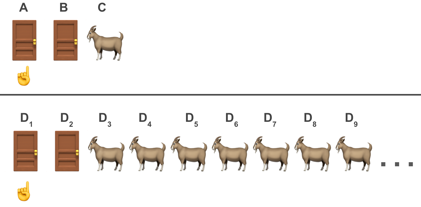
In both cases we had a prior belief that all doors had an equal chance of winning the prize p=1/N.
Once the host opened one door (N=3; or 98 doors when N=100) a lot of valuable information was revealed whereas in the case of N=100 it was much more apparent than N=3.
In the Frequentist approach, however, most of this information would be ignored, as it only focuses on the two closed doors. The Frequentist conclusion, hence is a 50% chance to win the prize regardless of what else is known about the situation. Hence the Frequentist takes Paul Erdős’ “no difference” point of view, which we now know to be incorrect.
This would be reasonable if all that was presented were the two doors and not the intervention and the goats. However, if that information is presented, one should shift gears into System 2 thinking and update their beliefs in the system. This is what we have done by focusing not only on the shut door, but rather consider what was learnt about the system at large.
For the brave hearted ⚔️, in a supplementary section below called The Bayesian Point of View I solve for the Monty Hall problem using the Bayesian formalism.
(4) Be one with subjectivity 🧘
The Frequentist main reservation about “going Bayes” is that — “statistics should be objective”.
The Bayesian response is — the Frequentist’s also apply a prior without realising it — a flat one.
Regardless of the Bayesian/Frequentist debate, as researchers we try our best to be as objective as possible in every step of the analysis.
That said, it is inevitable that subjective decisions are made throughout.
E.g, in a skewed distribution should one quote the mean or median? It highly depends on the context and hence a subjective decision needs to be made.
The responsibility of the analyst is to provide justification for their choices first to convince themselves and then their stakeholders.
(5) When confused — look for a useful analogy
... but tread with caution ⚠️
We saw that by going from the N=3 setup to the N=100 the solution was apparent. This is a trick scientists frequently use — if the problem appears at first a bit too confusing/overwhelming, break it down and try to find a useful analogy.
It is probably not a perfect comparison, but going from the N=3 setup to N=100 is like examining a picture from up close and zooming out to see the big picture. Think of having only a puzzle piece 🧩 and then glancing at the jigsaw photo on the box.
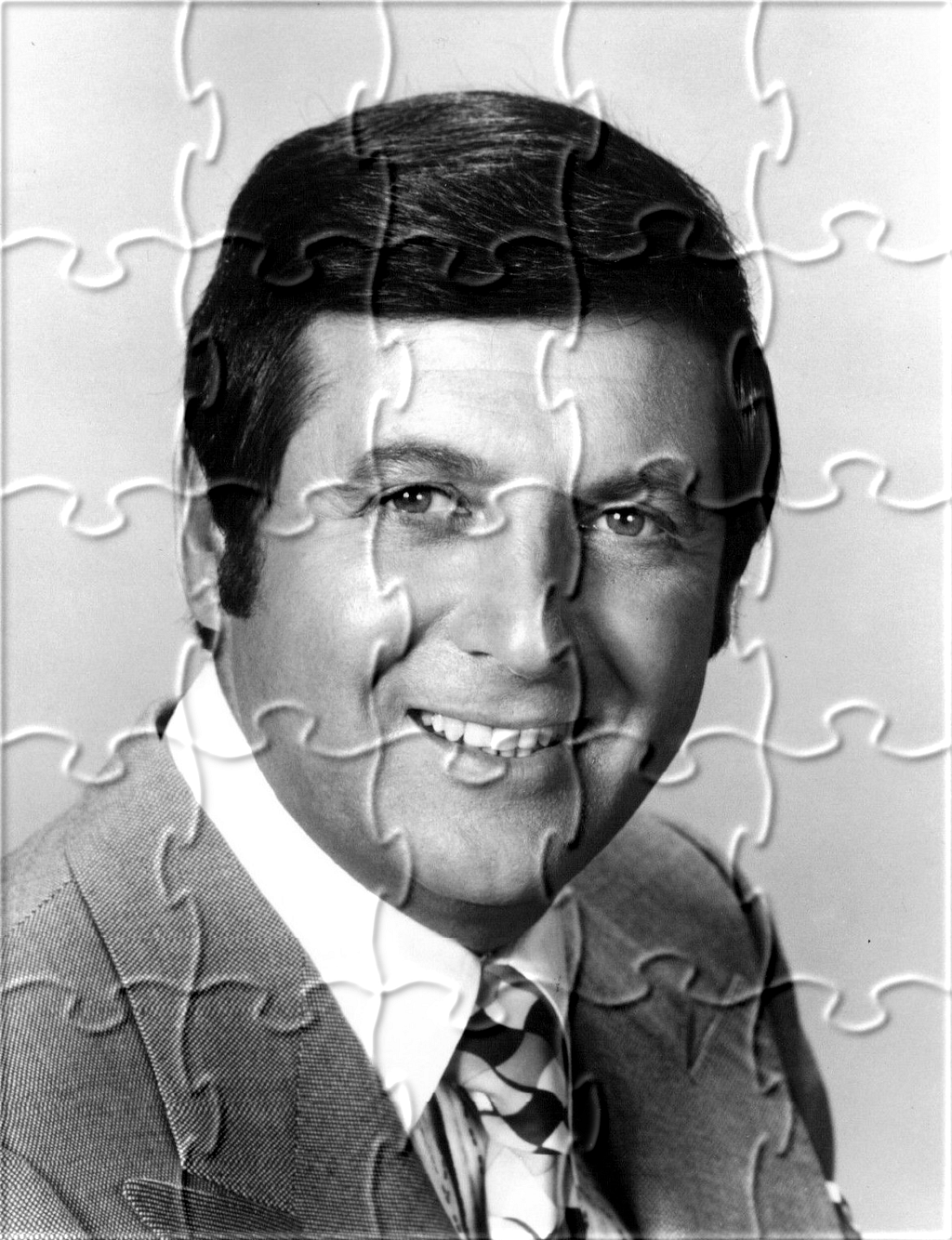
Note: whereas analogies may be powerful, one should do so with caution, not to oversimplify. Physicists refer to this situation as the spherical cow 🐮 method, where models may oversimplify complex phenomena.
I admit that even with years of experience in applied statistics at times I still get confused at which method to apply. A large part of my thought process is identifying analogies to known solved problems. Sometimes after making progress in a direction I will realise that my assumptions were wrong and seek a new direction. I used to quip with colleagues that they shouldn’t trust me before my third attempt ...
(6) Simulations are powerful but not always necessary 🤖
It’s interesting to learn that Paul Erdős and other mathematicians were convinced only after seeing simulations of the problem.
I am two-minded about usage of simulations when it comes to problem solving.
On the one hand simulations are powerful tools to analyse complex and intractable problems. Especially in real life data in which one wants a grasp not only of the underlying formulation, but also stochasticity.
And here is the big BUT — if a problem can be analytically solved like the Monty Hall one, simulations as fun as they may be (such as the MythBusters have done⁶), may not be necessary.
According to Occam’s razor, all that is required is a brief intuition to explain the phenomena. This is what I attempted to do here by applying common sense and some basic probability reasoning. For those who enjoy deep dives I provide below supplementary sections with two methods for analytical solutions — one using Bayesian statistics and another using Causality.
But first, let’s summarise the article by examining how, and if, the Monty Hall problem may be applied in real-world settings, so you can try to relate to projects that you are working on.
Application in Real World Settings
Researching for this article I found that beyond artificial setups for entertainment⁶ ⁷ there aren’t practical settings for this problem to use as an analogy. Of course, I may be wrong⁸ and would be glad to hear if you know of one.
One way of assessing the viability of an analogy is using arguments from causality which provides vocabulary that cannot be expressed with standard statistics.
In a previous post I discussed the fact that the story behind the data is as important as the data itself. In particular Causal Graph Models visualise the story behind the data, which we will use as a framework for a reasonable analogy.
➡️ Start Asking Your Data “Why?” - A Gentle Intro To Causality
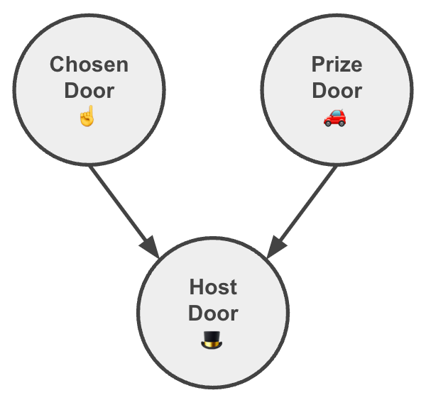
For the Monty Hall problem we can build a Causal Graph Model like this:
Reading:
- The door chosen by the trader☝️ is independent from that with the prize 🚗 and vice versa. As important, there is no common cause between them that might generate a spurious correlation.
- The host’s choice 🎩 depends on both ☝️ and 🚗.
By comparing causal graphs of two systems one can get a sense for how analogous both are. A perfect analogy would require more details, but this is beyond the scope of this article. Briefly, one would want to ensure similar functions between the parameters (referred to as the Structural Causal Model; for details see in the supplementary section below called ➡️ The Causal Point of View).
Anecdotally it is also worth mentioning that on Let’s Make a Deal, Monty himself has admitted years later to be playing mind games with the contestants and did not always follow the rules, e.g, not always doing the intervention as “it all depends on his mood”⁴.
In our setup we assumed perfect conditions, i.e., a host that does not skew from the script and/or play on the trader’s emotions. Taking this into consideration would require updating the Graphical Model above, which is beyond the scope of this article.
Some might be disheartened to realise at this stage of the post that there might not be real world applications for this problem.
I argue that lessons learnt from the Monty Hall problem definitely are.
Just to summarise them again:
(1) Assessing probabilities can be counter intuitive …
(Be comfortable with shifting to deep thought 🐢)
(2) … especially when dealing with ambiguity
(Search for clarity 🔎)
(3) With new information we should update our beliefs 🔁
(4) Be one with subjectivity 🧘
(5) When confused — look for a useful analogy … but tread with caution ⚠️
(6) Simulations are powerful but not always necessary 🤖
While the Monty Hall Problem might seem like a simple puzzle, it offers valuable insights into decision-making, particularly for data scientists. The problem highlights the importance of going beyond intuition and embracing a more analytical, data-driven approach. By understanding the principles of Bayesian thinking and updating our beliefs based on new information, we can make more informed decisions in many aspects of our lives, including data science. The Monty Hall Problem serves as a reminder that even seemingly straightforward scenarios can contain hidden complexities and that by carefully examining available information, we can uncover hidden truths and make better decisions.
At the bottom of the article I provide a list of resources that I found useful to learn about this topic.

Unless otherwise noted, all images were created by the author.
In the following supplementary sections ⚔️ I derive solutions to the Monty Hall’s problem from two perspectives:
- Bayesian
- Causal
Both are motivated by questions in textbook: Causal Inference in Statistics A Primer by Judea Pearl, Madelyn Glymour, and Nicholas P. Jewell (2016).
Supplement 1: The Bayesian Point of View
This section assumes a basic understanding of Bayes’ Theorem, in particular being comfortable conditional probabilities. In other words if this makes sense:

We set out to use Bayes’ theorem to prove that switching doors improves chances in the N=3 Monty Hall Problem. (Problem 1.3.3 of the Primer textbook.)
We define
- X — the chosen door ☝️
- Y— the door with the prize 🚗
- Z — the door opened by the host 🎩
Labelling the doors as A, B and C, without loss of generality, we need to solve for

Using Bayes' theorem we equate the left side as

and the right one as

Most components are equal (remember that P(Y=A)=P(Y=B)=⅓ so we are left to prove:

In the case where Y=B (the prize 🚗 is behind door B 🚪), the host has only one choice (can only select door C 🚪), making P(X=A, Z=C|Y=B)= 1.
In the case where Y=A (the prize 🚗 is behind door A ☝️), the host has two choices (doors B 🚪 and C 🚪) , making P(X=A, Z=C|Y=A)= 1/2.
From here

Quod erat demonstrandum.
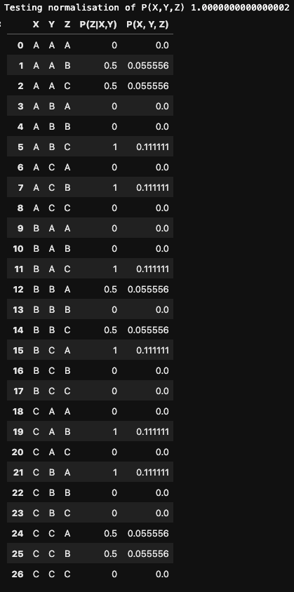
Note: if the “host choices” arguments didn’t make sense look at the table below showing this explicitly. You will want to compare entries {X=A, Y=B, Z=C} and {X=A, Y=A, Z=C}.
Supplement 2: The Causal Point of View ➡️
The section assumes a basic understanding of Directed Acyclic Graphs (DAGs) and Structural Causal Models (SCMs) is useful, but not required. In brief:
- DAGs qualitatively visualise the causal relationships between the parameter nodes.
- SCMs quantitatively express the formula relationships between the parameters.
Given the DAG

we are going to define the SCM that corresponds to the classic N=3 Monty Hall problem and use it to describe the joint distribution of all variables. We later will generically expand to N. (Inspired by problem 1.5.4 of the Primer textbook as well as its brief mention of the N door problem.)
We define
- X — the chosen door ☝️
- Y — the door with the prize 🚗
- Z — the door opened by the host 🎩
According to the DAG we see that according to the chain rule:

The SCM is defined by exogenous variables U , endogenous variables V, and the functions between them F:
- U = {X,Y}, V={Z}, F= {f(Z)}
where X, Y and Z have door values:
- D = {A, B, C}
The host choice 🎩 is f(Z) defined as:

In order to generalise to N doors, the DAG remains the same, but the SCM requires to update D to be a set of N doors Dᵢ: {D₁, D₂, … Dₙ}.
Exploring Example Scenarios
To gain an intuition for this SCM, let’s examine 6 examples of 27 (=3³) :
When X=Y (i.e., the prize 🚗 is behind the chosen door ☝️)
- P(Z=A|X=A, Y=A) = 0; 🎩 cannot choose the participant’s door ☝️
- P(Z=B|X=A, Y=A) = 1/2; 🚗 is behind ☝️ → 🎩 chooses B at 50%
- P(Z=C|X=A, Y=A) = 1/2; 🚗 is behind ☝️ → 🎩 chooses C at 50%
(complementary to the above)
When X≠Y (i.e., the prize 🚗 is not behind the chosen door ☝️)
- P(Z=A|X=A, Y=B) = 0; 🎩 cannot choose the participant’s door ☝️
- P(Z=B|X=A, Y=B) = 0; 🎩 cannot choose prize door 🚗
- P(Z=C|X=A, Y=B) = 1; 🎩 has not choice in the matter
(complementary to the above)
Calculating Joint Probabilities
Using logic let’s code up all 27 possibilities in python 🐍
df = pd.DataFrame({"X": (["A"] * 9) + (["B"] * 9) + (["C"] * 9), "Y": ((["A"] * 3) + (["B"] * 3) + (["C"] * 3) )* 3, "Z": ["A", "B", "C"] * 9})

df["P(Z|X,Y)"] = None
p_x = 1./3
p_y = 1./3

df.loc[df.query("X == Y == Z").index, "P(Z|X,Y)"] = 0
df.loc[df.query("X == Y != Z").index, "P(Z|X,Y)"] = 0.5
df.loc[df.query("X != Y == Z").index, "P(Z|X,Y)"] = 0
df.loc[df.query("Z == X != Y").index, "P(Z|X,Y)"] = 0
df.loc[df.query("X != Y").query("Z != Y").query("Z != X").index, "P(Z|X,Y)"] = 1

df["P(X, Y, Z)"] = df["P(Z|X,Y)"] * p_x * p_y

print(f"Testing normalisation of P(X,Y,Z) {df['P(X, Y, Z)'].sum()}")

df
yields
Resources
- This Quora discussion by Joshua Engel helped me shape a few aspects of this article.
- Causal Inference in Statistics A Primer / Pearl, Glymour & Jewell (2016) — excellent short text book (site)
- I also very much enjoy Tim Harford’s podcast Cautionary Tales. He wrote about this topic on November 3rd 2017 for the Financial Times: Monty Hall and the game show stick-or-switch conundrum
Footnotes
¹ Vazsonyi, Andrew (December 1998 — January 1999). “Which Door Has the Cadillac?” (PDF). Decision Line: 17–19. Archived from the original (PDF) on 13 April 2014. Retrieved 16 October 2012.
² Steve Selvin to the American Statistician in 1975.[1][2]
³Marilyn vos Savant’s “Ask Marilyn” column in Parade magazine in 1990
⁴Tierney, John (21 July 1991). “Behind Monty Hall’s Doors: Puzzle, Debate and Answer?”. The New York Times. Retrieved 18 January 2008.
⁵ Kahneman, D. (2011). Thinking, fast and slow. Farrar, Straus and Giroux.
⁶ MythBusters Episode 177 “Pick a Door” (Wikipedia)
⁶Monty Hall Problem on Survivor Season 41 (LinkedIN, YouTube)
⁷ Jingyi Jessica Li (2024) How the Monty Hall problem is similar to the false discovery rate in high-throughput data analysis.
Whereas the author points about “similarities” between hypothesis testing and the Monty Hall problem, I think that this is a bit misleading. The author is correct that both problems change by the order in which processes are done, but that is part of Bayesian statistics in general, not limited to the Monty Hall problem.
🚪🚪🐐 Lessons in Decision Making from the Monty Hall Problem was originally published in Towards Data Science on Medium, where people are continuing the conversation by highlighting and responding to this story.
from Datascience in Towards Data Science on Medium https://ift.tt/ZK6rwiU
via IFTTT


