
Machine Learning Model Selection: A Guide to Class Balancing
Comprehensive tutorial on class balancing for anonymized data for machine learning model selection

I’m bringing you a Machine Learning Model Selection project for Multivariate Analysis with Anonymized Data.
This is a comprehensive project where we’ll go from start to finish — from defining the business problem to the model deployment (though we’ll leave the deployment for another time).
There will be two full tutorials for this project, and I want to walk you through a range of techniques, including the added complexity of working with anonymized data — something increasingly common in the job market due to data privacy concerns.
So, what’s the big challenge with working on this type of data? It’s that you don’t have any information on what each variable represents.
Now, that’s tricky, isn’t it? You’ll receive the data, and without knowing what each variable stands for, you’ll need to develop a machine learning model from that.
We’ll also take this opportunity to dive into model selection. Which machine learning model will best help us make the predictions needed for this project? Is it possible to know beforehand which model is the best? No, it isn’t. I need to experiment.
We’ll try out a few models, compare them, and select the best one. The dataset we’re using was generated and anonymized by me. Once we have the best model, we’ll deploy it, use it to deliver predictions, and solve the problem it was created for.
Installing and Loading Packages
Let’s install and load the necessary packages. First, install the Watermark package to generate a watermark with the versions of the packages used.
For this tutorial, we only need three Python packages: the dynamic duo NumPy and Pandas to manipulate and preprocess the data.
# 1. Imports
import pandas as pd
import numpy as np
import pickle
Then, there’s the pickle package, which we’ll use to save the entire result of our work and the dataset to my GitHub. Once I finish this first part of the tutorial, I’ll grab the generated files, which are the result of our preprocessing, and continue later.
But why do we need pickle? We need it because I’ll be saving the column titles in a single file. You might be wondering — why save the column titles? This is a highly multivariate dataset with 179 columns. That’s a lot of columns.
To simplify the second part of the project, I’ll save the processed data along with the column titles in a single file. This will make our work much easier later on since we’re dealing with a dataset that’s packed with columns. The goal is to work with multivariate analysis.
So, let’s load all the packages, and then load Watermark next.
Loading the Data
Let’s load the dataset.
# 2. Loading the data
df = pd.read_csv("dataset.csv")
Now, let’s check the shape of the data.
# 3. Shape
df.shape
We have 11,500 rows and 179 columns — 178 columns of predictor variables and one column for the target variable.
Let’s take a quick look with head(). Here it is:
# 4. Viewing some records
df.head()
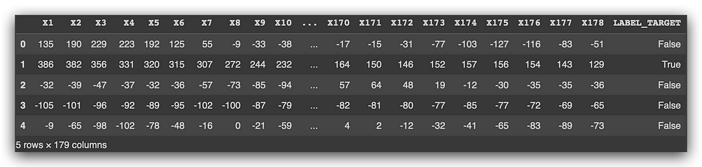
Let’s take a moment to look and understand what we have. You see several columns, with headers like x1, x2, all the way to x178. Then, you have values — some positive, some negative — and the target variable.
The data is anonymized, so you have no identification for the variables. Can we still work with this? Yes, of course we can. It’s not mandatory to know what each variable represents. Would it be ideal? Yes, because then I could do feature selection and check if any variables can be discarded.
We could still do that, but we’d only be looking at numbers without considering any domain knowledge.
Here’s the approach: the data has already been filtered and anonymized. All we’ve been asked to do is create a machine learning model. Once the model is ready, someone will feed it with 178 characteristics of a client, and they’ll want the model to produce a prediction. That’s it.
So, your job isn’t to interpret the variables — not in this case. You don’t have the titles of the variables, nor the data dictionary. We have absolutely nothing.
But that’s not our task right now. We’re here to build the model. That’s what we’ve been asked to do, and that’s exactly what we’re going to accomplish.
Even so, we’ll make some checks, and then build the machine learning model. Once the model is ready, whoever uses it will need to feed it with 178 anonymized input variables. My job is to take this information and try to build a model from it.
This is a genuine data science project.
Exploratory Data Analysis and Data Cleaning
Let’s start with some exploratory data analysis to check if there are any issues. If necessary, we’ll also clean the data as we go.
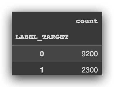
We’ll begin by checking the categories of the target variable, which is LABEL_TARGET. This variable essentially represents whether a customer renewed their car insurance or not. We have historical data that we’ll use to build the machine learning models.
So, let’s count the number of records for each category.
# 5. Categories of the target variable
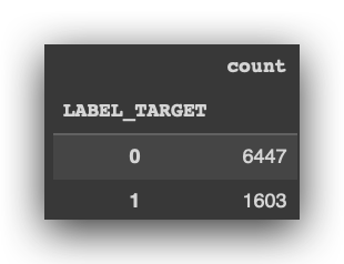
df.LABEL_TARGET.value_counts()
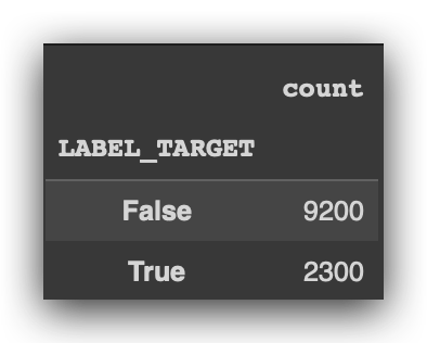
In this case, we have two categories: false and true. False means the customer did not renew their insurance, while true means they did.
What do you notice? There’s a much larger number of records in the false class than in the true class. This is a problem. Why? Because the data is imbalanced.
Now, there’s nothing wrong with the data itself. It’s normal to have more records in one class than in the other. That’s fine. But the machine learning model doesn’t understand what a class is, it doesn’t know what a category is, nor does it understand concepts like cars or insurance. The model only knows math.
So, I need to provide the model with a similar proportion of records for each class — at least something close. If I feed the data in its current state, what will happen? The machine learning model will learn much more from the false class than from the true class.
When I use the model to predict new data, it will likely predict false more accurately than true. And that’s not good. I want a balanced model.
This is why exploratory analysis is important — to detect these kinds of issues. We’ll resolve this soon.
Next, let’s convert this variable from a categorical type (currently in text form) to an integer type.
# 6. Convert from string to numeric value
df["LABEL_TARGET"] = df["LABEL_TARGET"].astype(int)
Because machine learning is just math, we’ll go ahead and make the conversion now. I’m using astype(int) for this.
Now, observe the result: 0 and 1.
# 4. Viewing some records
df.head()
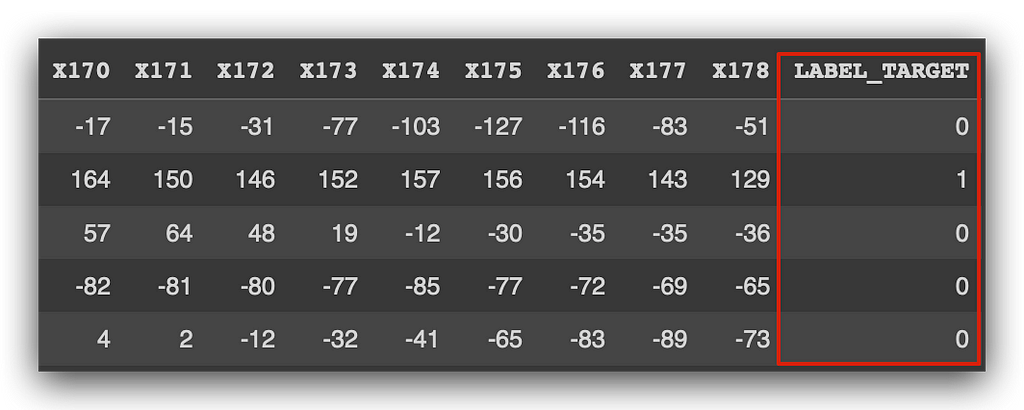
0 represents the negative class, and 1 represents the positive class. In the negative class, the event didn’t happen; in the positive class, the event did happen. And what is the event? Renewing car insurance.
What we’ve done here is modify the data without changing the information. Is the information the same? Yes. Is the data different? Yes, and that’s fine. You can modify the data, but you cannot change the information.
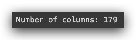
Let’s now check the exact number of columns to ensure everything is correct.
# 7. Print the number of columns
print("Number of columns:", len(df.columns))
Let’s generate a statistical summary using the describe method. What does it do? It calculates the mean, standard deviation, minimum value, first quartile, second quartile (which is the median), third quartile, and the maximum value.
It performs these calculations for each of the variables.
# 8. Statistical summary
df.describe()
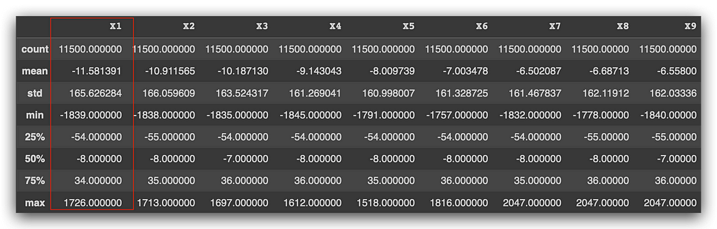
Now, we’ll have to make some decisions. Take a look at the variable X1, for example. We don’t know what it represents — it’s a client characteristic, but I wasn’t told what it is because I’m not supposed to know. The data is anonymized.
The mean is -11, standard deviation is 165, and the minimum value is -1839. Then, we have the median and the maximum value. Without knowing what the variable represents, it’s hard to interpret whether these values are coherent or not. I was told that, yes, the values are coherent.
Now, I could check for outliers using a standard statistical approach. I’d verify the interquartile range, identify the outliers, and remove any values above the maximum or below the minimum. However, since I’ve been told that the data has already been filtered and validated, I’m not going to apply any outlier detection or treatment strategies.
Later, I’ll standardize the data, putting everything on the same scale. If there happens to be an outlier, I’ll bring it back to the center and place it on the same scale. That’s my decision.
In this case, I’ve been informed that the data is already filtered and validated. So, I won’t worry about outliers. If there’s anything affecting the model’s training, I’ll address it during standardization. Sound good?
But we do need to check for missing values. If there are any, we have no choice but to resolve them. Missing values are a problem. If I leave them in the dataset, it will affect the calculations, and I won’t even be able to train the model — it will cause errors.
# 9. Checking for missing values
df.isnull().values.any()

False — No missing values. But you should always do the check. Remember that, okay?
# 10. Extract the list of columns
column_list = df.columns.tolist()

# 11. Input variable columns
input_columns = column_list[0:178]

print(input_columns)
Here, we’re extracting the list of columns. There are a lot of columns, and I’ll use this as the input columns.


Take a look at the number of columns we have here, ranging from X1 to X178. This is a highly multivariate dataset. So, I’ll check if there are any duplicate columns in the input data. When you have a dataset like this, with so many variables, it’s not enough to just try and spot duplicates visually.
Let’s check for duplicate columns, as it can happen.
# 12. Checking if there are duplicate columns in the input data
dup_cols = set([x for x in input_columns if input_columns.count(x) > 1])
print(dup_cols)
assert len(dup_cols) == 0, "You have duplicated columns in input_columns"
What is a duplicate column in this case? It’s a column that shares the same name. Someone might have made an error while preparing the dataset, so we’ll check for this.
I’m using set, which is a collection in Python, along with list comprehension. Let’s break it down: for each value x in the input columns, if the count of that column is greater than 1, or if I have more than one occurrence of the column, I’ll return x.
If I don’t return anything, it means I have no duplicates.
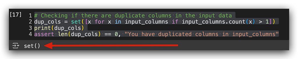
Execution done. Empty — no duplicate columns.
Now, let’s check if we have any duplicate columns in the complete dataset.
# 13. Checking if there are duplicate columns in the complete dataset
dup_cols = set([x for x in column_list if column_list.count(x) > 1])
print(dup_cols)
assert len(dup_cols) == 0, 'You have duplicated columns in column_list'
Notice that earlier I used input_columns, and now I’m using column_list. I’ll perform the same check.
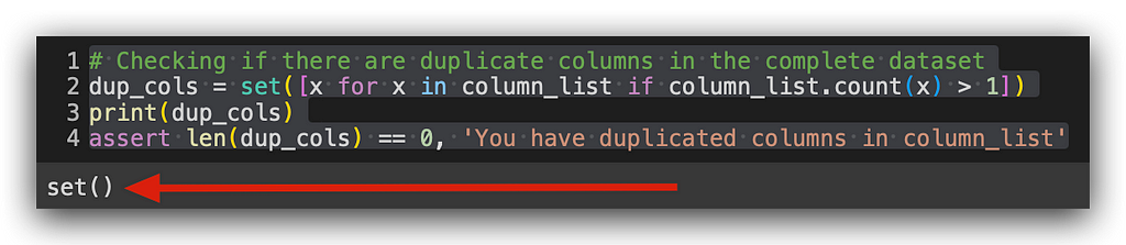
Empty again — no duplicates here either. Now, let’s look at the categories of the target variable.
# 14. Categories of the target variable
df.LABEL_TARGET.value_counts()
In exploratory analysis, we’re primarily looking for patterns in the data and any potential issues, like missing values or outliers. From there, we make decisions.
Missing values — those have to be handled. There’s no way around that. As for outliers, well, you have a choice. You can either keep them and resolve the issue later during standardization, or you can identify and address them immediately. Both options are valid.
Pick one, document your decision, and move forward with your process.
Now, since we have a clear difference in the number of records between class 0 and class 1, let’s calculate the prevalence of the positive class. How do we do that? Let me run the code for you first — it’ll make things easier to understand.
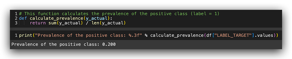
# 15. This function calculates the prevalence of the positive class (label = 1)
def calculate_prevalence(y_actual):
    return sum(y_actual) / len(y_actual)

print("Prevalence of the positive class: %.3f" % calculate_prevalence(df["LABEL_TARGET"].values))
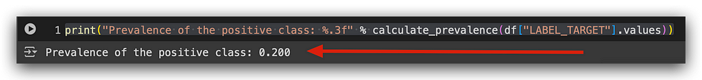
The prevalence of the positive class is 0.2, or 20%. What does this mean? In our total sample, which is our dataset, 20% of the records belong to the positive class. In other words, 20% of the people renewed their car insurance. Consequently, 80% belong to the negative class — those who did not renew.
The dataset is heavily imbalanced, and this poses a problem when training most machine learning models. We have a much larger proportion of one class over the other. It doesn’t have to be a perfect 50/50 balance. It could be 52/48 or 55/45. Even 60/40 is a reasonable proportion.
However, an 80/20 split is too large of a difference. This naturally creates problems because you’re giving the model far more examples from one class than the other.
Think of it this way: if you’re learning math and geography, and you do way more math exercises than geography, which subject will you learn better? Math, of course — you’ve had more examples. The same concept applies here.
If I provide the dataset to the model in its current form, it will learn far more from the negative class than the positive one, simply because the difference in examples is so large. This is a problem, and it needs to be addressed.
Some algorithms can handle data in this format and still learn without major issues, but these are few. The more common algorithms expect to receive data in at least a somewhat balanced proportion.
So, I’ll now teach you how to handle class balancing. But, before balancing, we need to split the data into training, testing, and validation sets.
Balancing is applied only to the training data. You don’t need to apply it to the validation and test data. Does that make sense? That’s why I have to split the dataset into training, validation, and test samples first. Once the dataset is split, I’ll balance the training data, train the model, and we’re done.
When the model is trained, I’ll use the validation and test data, and at that point, balancing doesn’t matter. I just want the model to make predictions, that’s all.
First, I’ll generate random samples from the data. Pay attention, because there’s a detail here: I’ll generate random samples using the sample function.
# 16. Generating random samples from the data
df_data = df.sample(n = len(df))
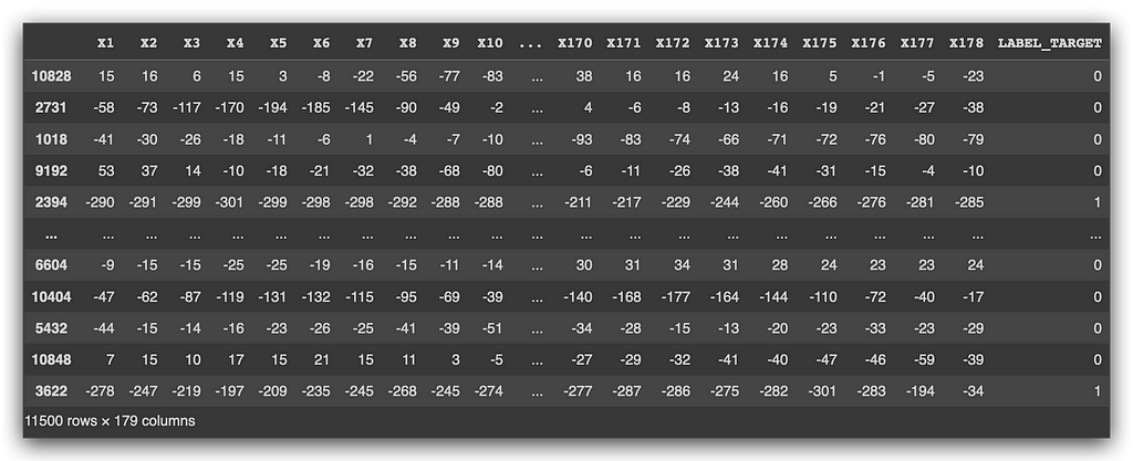
Let’s generate a random sample, and here’s the data. Notice the index, which is the bolded part on the left — this is the Pandas index. I took the original dataset and shuffled the data to make it as random as possible. This ensures that the samples are created randomly, which is the essence of random sampling, a statistical technique.
Now, even though the data has already been shuffled, and everything looks good, I need to adjust the index. Otherwise, I won’t be able to perform the split the way I want.
Whenever you modify a Pandas DataFrame, it’s best to reset the index afterward.
# 17. Adjusting the dataset indices
df_data = df_data.reset_index(drop=True)

df_data
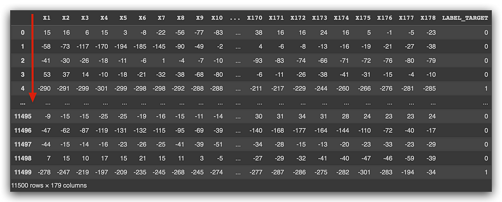
Run the command and take a look at the result. The data is still random, but I’ve adjusted the numbering. When you load data, Pandas automatically assigns an index for you. I changed the order of the data, shuffled everything, and naturally, the index was shuffled too.
What I’ve done is simply rebuild the index, because I’m going to use it for the data split. After that, I’ll use the samplefunction once again to extract a 30% sample of the data (0.3). This sample will be extracted randomly from the dataset, creating a new DataFrame.
# 18. Extracting a 30% random sample from the data
df_sample_30 = df_data.sample(frac=0.3)

print("Validation/Test split size: %.1f" % (len(df_sample_30) / len(df_data)))
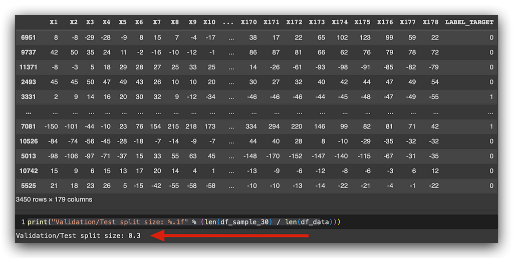
Take a look at the total — 3,451 rows, which represent 30% of the original DataFrame. At this point, I’ve split the data 70/30. I’ll keep 70% of the data for training, and I’ll split the remaining 30% into two subsamples: 15% for testing and 15% for validation.
So, first, I’ll check the size of the split (which we’ve done with the 0.3 sample), and now I’ll continue splitting it further. From df_sample_30, which contains 30% of the data, I’ll divide it into two equal parts—50% for testing.
# 19. Performing the split

# Test data
df_test = df_sample_30.sample(frac=0.5)

# Validation data
df_valid = df_sample_30.drop(df_test.index)

# Training data
df_train = df_data.drop(df_sample_30.index)
Next, I’ll drop the rows that I’ve already assigned to the test set. The rest will go into the validation set. Then, I’ll take the remaining 70% and assign it to the training set.
So, I’ve just completed the split into test, validation, and training sets. Here’s what we have:
- The test dataset contains 1,725 rows, representing 15% of the total.
- The validation dataset also contains 1,725 rows, representing 15%.
- The training dataset contains 8,050 rows, which represent 70% of the total.
Now, this random sampling and split had an additional purpose. Besides dividing the data into training, test, and validation sets, I also carried over the prevalence of the positive class. In the original dataset, 20% of the records belong to the positive class, and 80% to the negative class.
Imagine if I hadn’t been careful when splitting the data into training, validation, and test sets. If I had done the split carelessly, this is what could happen…
These 20% of records from the positive class could have ended up entirely in the validation and test sets — all 20% in validation and test, while the remaining 80% would be, for example, in the training set and partly in validation.
In other words, I could have risked training the model only on data from one class and then evaluating it with data from the other class. If I don’t take care to carry this prevalence into the subsamples we’re creating, I run the risk of making this problem even worse — potentially having only one class in the training set and the other class in test and validation.
This would create two totally different samples with very different data patterns, which would obviously cause significant problems.
That’s why, when splitting the data, we must be careful to preserve the prevalence. And what strategy did I adopt to do this? Random sampling.
# 16. Generating random samples from the data
df_data = df.sample(n = len(df))
Random sampling works very well, and all you need to do in Python is use the sample method from the Pandas DataFrame. It applies random sampling and works amazingly well—that’s all you need to do.
# 20. Check the prevalence of each subset
print(
    "Test (n = %d): %.3f"
    % (len(df_test), calculate_prevalence(df_test.LABEL_TARGET.values))
)
print(
    "Validation (n = %d): %.3f"
    % (len(df_valid), calculate_prevalence(df_valid.LABEL_TARGET.values))
)
print(
    "Train (n = %d): %.3f"
    % (len(df_train), calculate_prevalence(df_train.LABEL_TARGET.values))
)
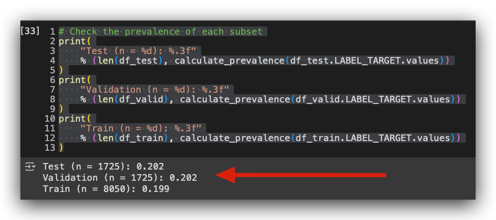
Take a look at the result. I now have 20% of the positive class in the test set, 20% in the validation set, and 20% in the training set. In other words, I preserved the original prevalence of the data when performing random sampling for the subsamples.
All I needed to do was use the sample function, which applies random sampling—a fundamental statistical technique. We’ve maintained the same representation and pattern in the subsamples as we had in the original data.
If I hadn’t taken this precaution, I could have ended up with, for example, 95% of the positive class in the test set and 0% in the training set. If that happened, there wouldn’t even be a need for class balancing, as everything would be concentrated in a single class. This would have caused a massive problem.
So, when working on classification problems like ours, and you encounter a significant discrepancy in the class prevalence — like we do here — use random sampling to create your training, validation, and test sets.
Random sampling usually carries this proportion forward into the subsamples, but it’s always good to verify, just like we did here. I checked whether the proportion was appropriate for each subsample, formatting the result with three decimal places (hence the %.3f formatting). In this way, we’ve carried the pattern from the original data into the subsamples. Excellent!
However, to train the model, I now need to apply class balancing. We’ve split the data as we did, and now I’ll balance the training data. From there, I’ll train the model. Once the model is trained, I’ll then validate it and test it using data with the correct proportion.
This is the ideal approach when working on classification problems, especially when there’s a large discrepancy in the prevalence of the positive class — which is the event you’re trying to predict.
Class Balancing
When it comes to class balancing, we have various strategies, techniques, and tools available. For this tutorial, I’ll introduce one specific strategy — undersampling. This means I’ll be reducing the majority class.
Let’s take a look at the shape of the test, validation, and training sets.
# 21. Check the shape of the datasets and value counts
# of the target variable in the training set

df_test.shape

df_valid.shape

df_train.shape

df_train.LABEL_TARGET.value_counts()
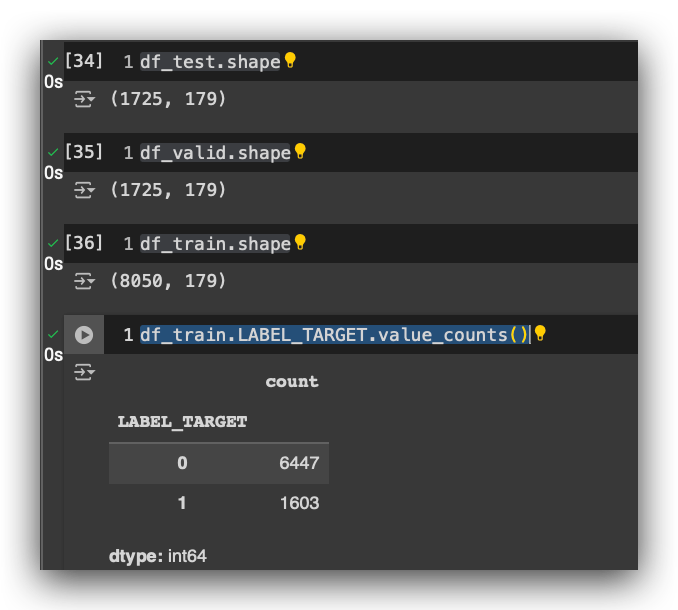
Let’s count the proportion of the target variable in the training data. As you can see, we’ve maintained that 80–20 proportion. We have far more examples of class 0 (customers who didn’t renew their insurance) than of class 1(customers who renewed).
If I were to apply oversampling, I’d need to use a technique to increase the size of the minority class. What’s the minority class? It’s class 1 — the customers who renewed their insurance. In general, a statistical technique would be applied to the class 1 data to generate synthetic samples (synthetic values) and increase the size of the minority class. That’s what oversampling is.
Undersampling, on the other hand, is the opposite. I’ll reduce the majority class, which in this case is class 0.
Both strategies have their pros and cons, like most things in life. If I used oversampling, what would happen? I’d end up creating nearly 4,000 synthetic records — just over 4,000, to be more precise. Agree? I’d have to add records to class 1 to bring it closer to the size of class 0. It doesn’t need to be exactly equal, but at least close.
So, I’d have to create a large number of synthetic records. This is a disadvantage because, in practice, I’d be creating data. Although it’s done through a statistical procedure, the large quantity of generated data would be purely synthetic.
On the other hand, oversampling gives you more data to train the model, which is an advantage.
Now, undersampling. I won’t need to create synthetic data. Instead, I’ll delete records from the majority class. So, I won’t be creating new data; I’ll be removing it. This is an advantage because I’m not introducing synthetic data. However, the disadvantage is that I’ll lose data.
It’s like the story of a short blanket — cover your head, and your feet are exposed, and vice versa. So, what’s the decision? You have to choose and move forward, always documenting and justifying your decision. There’s no way to know right now what the ideal decision is. I’ll only know later when I evaluate the model. The model evaluation will tell me if I made the right choices.
Since I haven’t built the model yet, there’s no way to know for sure. But I need to make a decision to create the model.
I’m going to choose undersampling. I’ll justify my decision: If I used oversampling, I’d have to create a massive amount of synthetic data, which could potentially alter the data’s characteristics significantly. I might end up creating a pattern that doesn’t exist, which would later harm the model’s balance.
So, I won’t use oversampling. I’d rather lose some data than create synthetic data. In this case, the discrepancy is too large. If the difference were smaller, say 60–40, and I had to use oversampling, it would be different because I wouldn’t need to create as many synthetic records. Agree?
But here, the difference is 80–20. To equalize the classes, I’d need to generate a massive amount of synthetic data, and I’d likely end up creating patterns that don’t exist.
However, I can only be sure if I test it. So, what am I going to do? I’ll apply undersampling. Later, I’ll evaluate the model and see if this was a good decision or not. If it wasn’t effective, I’ll go back and change my approach — no problem at all. You can always change your decision later, based on the information you have at the time.
Since I need to balance the data to train the model, this is a decision I can’t postpone — it has to be made now. I’ll go with undersampling, and I’ve just justified my reasoning. I don’t want to create such a large volume of synthetic data. I’d rather lose some data, even if it means losing a bit of the pattern.
But by doing so, I won’t be introducing synthetic data. That’s my choice, and I’ve just justified it. Let’s apply it, and later we’ll evaluate the model to see if it was the right call.
Now, let’s create an index with true or false, and I’ll use this index to define the positive and negative values.
# 22. Create an index with True/False
index = df_train.LABEL_TARGET == 1

# 23. Define positive and negative values from the index
df_train_pos = df_train.loc[index]
df_train_neg = df_train.loc[~index]
I’ll use this to remove the data I don’t want from the majority class. I’ll define df_train_pos for the positive class and df_train_neg for the negative class.
After that, I’ll calculate the minimum number of records between the positive and negative classes.
# 24. Minimum value of records between positive and negative classes
min_value = np.min([len(df_train_pos), len(df_train_neg)])

min_value
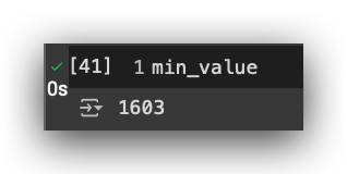
Ideally, you should have at least 1,603 records in class 0. It doesn’t need to be exactly equal, but at least 1,603, so you don’t delete records from the minority class. I want to delete records from the majority class, while preferably keeping everything we have in the minority class.
If I happen to need to delete some records from the minority class, that’s okay, but always be careful with that.
Let’s now check the minimum number of records. After that, we’ll get random values for the training dataset, always using random sampling with the sample function.
# 25. Get random values for the training dataset
df_train_final = pd.concat([df_train_pos.sample(n = min_value, random_state = 69),
                            df_train_neg.sample(n = min_value, random_state = 69)],
                           axis = 0,
                           ignore_index = True)
So, what I’ll do here is actually quite simple. Out of the 6,447 records, I’ll randomly select 1,603 and keep them in class 0, discarding the rest.
By selecting the data randomly, you avoid losing any significant patterns, though some data loss is always possible.
# 26. Random sampling of the training dataset
df_train_final = df_train_final.sample(n = len(df_train_final), random_state = 69).reset_index(drop=True)

df_train_final.shape
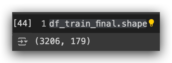
After that, we’ll perform random sampling on the training dataset. Once the sampling is done, here’s the shape: 3,206 rows and 179 columns.
Next, let’s check the class proportion.
# 27. Check value counts of the target variable in the final training set
df_train_final.LABEL_TARGET.value_counts()
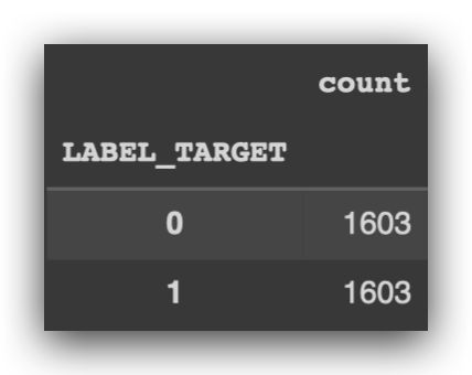
And there it is: 1,603 records for class 1 and 1,603 for class 0. What I did for the undersampling was to randomly select 1,603 records from the majority class, discard the rest, and now the classes are balanced.
This is something you only do for the training data — just to train the model. For the validation and test data, it’s not necessary, because the model has already been trained.
# 28. Dataset balancing
print('Balance in Train (n = %d): %.3f' % (len(df_train_final),
                                           calculate_prevalence(df_train_final.LABEL_TARGET.values)))
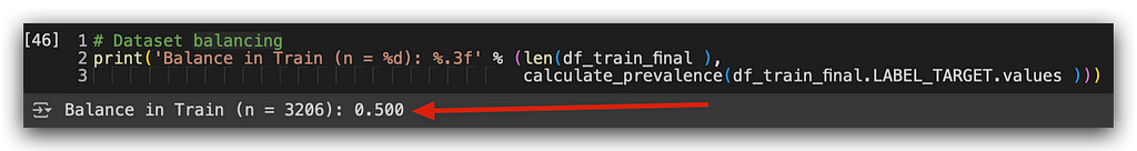
Let’s check the class balance now. Done! I now have a 50–50 proportion. It’s not mandatory to have an exact 50–50 balance, but something close to it is ideal.
We can now wrap up our work by saving everything we’ve done so far to disk.
Saving the Preprocessing Results
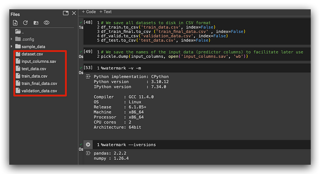
We’ve prepared the training data, the final training dataset, as well as the validation and test datasets. There’s no need to include the index, so the index is set to False.
# We save all datasets to disk in CSV format
df_train.to_csv('train_data.csv', index=False)
df_train_final.to_csv('train_final_data.csv', index=False)
df_valid.to_csv('validation_data.csv', index=False)
df_test.to_csv('test_data.csv', index=False)
The data has been successfully generated. This means you can have one notebook dedicated to data processing, and another one dedicated to modeling. You could create this notebook as a template for your day-to-day work. One Jupyter Notebook could contain the strategies you use to process the data, while another could focus on the modeling part.
Let’s also save the input columns — remember those? The titles? When loading the data later, I’ll use these input columns in the exact order I defined during preprocessing.
# We save the names of the input data (predictor columns) to facilitate later use
pickle.dump(input_columns, open('input_columns.sav', 'wb'))
So, I’ll save it in SAV format, which is the format used by pickle. And with that, we conclude the preprocessing stagefor a dataset with a large number of variables and anonymized data.
This wraps up the first part of our work on this project.
What will I do in the next tutorial?
I’ll take the data I’ve shown in the image, and we’ll train multiple machine learning models. We’ll train models with hyperparameters, without hyperparameters, apply cross-validation, use different algorithms, and evaluate the models with various metrics. Then, we’ll choose the best model and deploy it.
We’ll solve the business problem, deliver the project to the client, make the client happy, and move on to the next one.
Review everything we’ve done in this tutorial, and join me as we create the long-awaited machine learning models!
Thank you very much. 🐼❤️
All images, content, and text are created and authored by Leonardo Anello
Machine Learning Model Selection: A Guide to Class Balancing was originally published in Towards Data Science on Medium, where people are continuing the conversation by highlighting and responding to this story.
from Datascience in Towards Data Science on Medium https://ift.tt/vaxSKCV
via IFTTT


