
PyTorch Optimizers Aren’t Fast Enough. Try These Instead
These 4 advanced optimizers will open your mind.
If you’ve been working with deep learning for a while, you’re probably well-acquainted with the usual optimizers in PyTorch — SGD, Adam, maybe even AdamW. These are some of the go-to tools in every ML engineer’s toolkit.
But what if I told you that there are pleanty of powerful optimization algorithms out there, which aren’t part of the standard PyTorch package?
Not just that, the algorithms can sometimes outperform Adam for certain tasks and help you crack tough optimization problems you’ve been struggling with!
If that got your attention, great!
In this article, we’ll take a look at some advanced optimization techniques that you may or may not have heard of and see how we can apply them to deep learning.
Specifically, We’ll be talking about Sequential Least Squares ProgrammingSLSQP, Particle Swarm Optimization PSO, Covariant Matrix Adaptation Evolution StrategyCMA-ES, and Simulated Annealing SA.
Why use these algorithms?
There are several key advantages:
- They are all gradient-free optimization techniques, meaning your code doesn’t even need to be differentiable! So, you can work with non-differentiable operations such as sampling, rounding, step functions, and combinatorial options, as well as hyperparameters, which have complex effects on performance that are hard to understand.
- You only need to compute the forward pass to make them work, so these methods can be faster and require less GPU memory. There is no need to implement custom backward functions and straight-through estimators (STEs).
- Most of them are global optimization methods, meaning that even if you get stuck in many suboptimal local minima, these algorithms won’t be confused and will find the best global minima. (Given enough time).
One caveat:
The approaches we will look at work best for a small number of parameters to optimize; somewhere less than 100–1000 is reasonable. Any more than that and these algorithms may run into errors or just never converge.
So, it is best to use it to optimize key parameters, such as prediction heads, special parameters per layer, or hyperparameters.
That said, if your problem fits these characteristics, or if you’re just looking to get an extra edge with your neural networks. These optimization algorithms might be exactly what you need when traditional methods fall short.
Before We Start
Let’s first set up our imports, helper functions, and common variables. We’ll be using these a lot down the line.
Imports and Helper Functions
You’re probably saying to yourself: “Can’t he just get to the algorithms already?”.
Well, no.
I want this post to be complete in the sense that it will provide you with:
- Usable code that you can copy, and it will run out of the box.
- The ability to reproduce my results.
Back to the boring imports.
Here, we want to import some libraries we will use for optimization, data handling, logging, and visualizing the optimization process.
We also set the seeds for reproducibility.
In addition to the imports, we will define three essential helper functions:
- set_model_weights_from_vector() This function will take in our neural network and a numpy 1d arraycontaining the “flattened” weights and biases of the layers of the neural network.
This is the vector we will optimize — as it contains the model weights and biases.
This function will then parse this vector and insert it as the weights and biases of the model. - get_vector_from_model_weights() This function does the opposite; it parses the weights and biases from the model and flattens them into a numpy 1d array.
- update_tracker() This just manages the tracking of the “best so far” loss values since this is what all the algorithms return.
Objective Functions
What are these?
So, most optimization algorithms refer to the “value we want to optimize” as the “objective function.” In deep learning, we typically call this thing as the loss function, which calculates the error between targets and predictions.
However, in most other optimization algorithms, the interface is different.
The main input to the objective function are the parameters we want to optimize such that we minimize (or maximize) the value of the objective function.
That said, it is very common to have additional arguments, which in our case include the model, input, target, and some other things for tracking the loss values.
Here, we also define a similar interface for the PyTorch optimization loop to compare the different optimizers.
The argument maxiter, is the number of optimization steps our algorithms will be allowed to take, and we will be the same across all algorithms.
We’ll set this to 100, since we want very fast optimization here.
Common Variables
Are we done yet?
Almost.
The last thing we need to do is define our super simple 2-layer neural network, as well as the inputs, targets, initial weights, etc.
A few things to note:
- We convert the input and target to double, i.e. torch.float64. This is to make it compatible with numpy vectors that have the precision expected by the other optimization algorithms.
- We intentionally make the input and target have different sensitivities (in line 3, we multiply by 1e3). This is to make the optimization problem harder so that we can see the contrast in performance between the methods. This is also called making the problem “ill-conditioned.”
- We intentionally make the network “small” so that the optimization process runs faster. Also, recall that these methods won’t work well if the number of parameters to optimize exceeds, say, 1000.
1. PyTorch Optimization With Adam
Ready? Let’s go!
The first item on our list will be our baseline, here we will just call run the super simple PyTorch optimization loop we defined before. We will use Adam, with a relatively large learning rate of 1., since this is what I found gave the best performance.
After running this, you should get this output.
Final loss Adam optimizer: 91.85612831226527
Not bad for 100 optimization steps, considering the initial loss value was around 300,000!
2. Sequential Least Squares Programming (SLSQP)
What is this jibberish?
This is actually one of the coolest, easiest-to-use, and fastest optimization algorithms you’ll find out there, especially if the problems you are trying to solve have continuous parameters and aren’t that hard.
Sequential Least Squares Programming (SLSQP) is like a smart puzzle solver that tries to fit all the pieces perfectly while obeying strict rules.
It tries to model your problem as a parabola (which has a single minima), but in many dimensions, based on the local information from samples around your initial guess x0.
Then, at each step, it moves to the minima of the parabola and remodels it based on the new local information. Lastly, rinse and repeat until it no longer improves the value of the objective function or until it reaches the maximal number of steps maxiter.
The main advantage of this approach is that it is great at handling constraints on your parameters if you have any. But also, in general, it converges really fast!
When running this algorithm, you should get the following output:
Final loss slsqp optimizer: 3.097042282788268
Already an improvement! And when we visualize this later, you’ll see that it reaches this value very fast.
3. Particle Swarm Optimization (PSO)
Now this sounds cool!
Imagine optimization without gradients. Sounds impossible, right? But that’s exactly what Particle Swarm Optimization PSO and the rest of the algorithms here do!
PSO is a population-based algorithm inspired by how birds fly in flocks, or fish swim in schools — basically, particles (potential solutions for the parameters to optimize) move around the solution space based on:
- their own experience and
- their neighbors’ experiences.
This algorithm doesn’t care about gradients — it shines in non-differentiable or noisy problems where gradient-based methods like Adam fail. It is also especially good for optimization problems that have many local minima.
I used PSO several times for hyperparameter tuning, and it worked pretty fast, though it sometimes requires its own hyperparameter tuning. You’ll be surprised, but this method might actually work really well for you!
Let’s take a look at the code:
Note that we need to define the upper bound ub and lower bound lb for each of the parameters. This is to make sure the algorithm doesn’t go too crazy with searching around for good values.
When running this, you should get the following output:
Final loss pso optimizer: 1.0195048385714032
Even a bit better than the previous method.
4. Covariance Matrix Adaptation Evolution Strategy
This method is just bonkers!
I first ran into this method when I was researching genetic algorithms.
This algorithm is from 1996 and is still considered state-of-the-art in hard optimization problems!
The Covariance Matrix Adaptation Evolution Strategy CMA-ES is an evolutionary algorithm that is designed for the hardest and toughest optimization problems. I’m talking about non-convex, discontinuous, noisy problems with many local minima!
CMA-ES is self-adapting, meaning it continuously updates its strategy based on the information it learns about your problem. It uses many samples and a population to probe and learn which parameters work best. This gradually improves its process of generating new populations in each iteration.
I’ve personally used CMA-ES in my research, and so have many others! It truly is the gift that keeps on giving since this algorithm is super versatile, battle-tested in many scenarios, and still stands the test of time!
I highly recommend it!
When running this code, you should get the following output:
(5_w,10)-aCMA-ES (mu_w=3.2,w_1=45%) in dimension 10 (seed=42, Thu Oct 10 22:03:53 2024)
Final loss cma optimizer: 4.084718909553896
Since it can converge sometimes a bit slow, and we don’t give it many samples, it doesn’t reach super great performance, though still better than Adam.
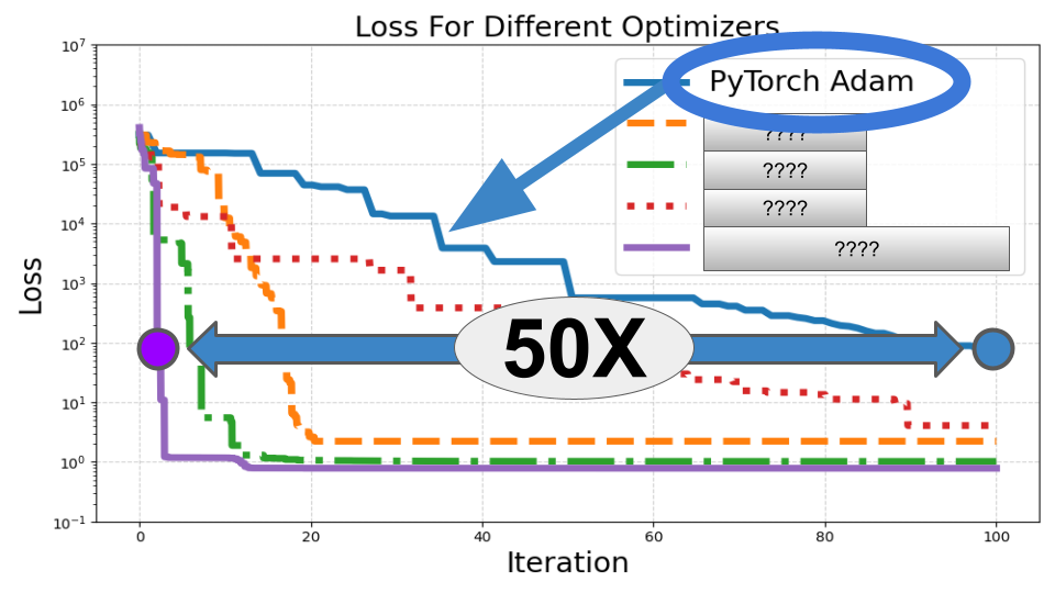
5. Simulated Annealing (SA)
This one is a classic and 50X faster than Adam in this demo!
Finally, let’s talk about Simulated Annealing SA.
If you’ve ever felt like your optimizer was trapped in a local minimum, this algorithm’s for you.
SA was initially inspired by physical processes such as cooling metal and quantum tunning.
Early on, the algorithm is “hot,” meaning it’s willing to explore many potential solutions for the parameters to optimize, even if they have worse objective function values. Later, the algorithm “cools,” and it becomes more conservative about accepting worse solutions, causing it to converge.
Dual Annealing combines both global search to look for different local minima, as well as local search to find the bottom of each local minima. This let’s it “consider” many different local minima until it finds the best one.
What I love about SA is its ability to escape bad local minima. Some argue it is outdated compared to more modern evolutionary algorithms, but I’d disagree — it’s still a great option where traditional optimizers fail, and it is definitely worth a try. It is also highly parallelizable, making it easily scalable to very large numbers of samples.
When running this code, we will get the following output
Final loss simulated_annealing optimizer: 0.7834294257939689
This is the best result we got so far! And as we can see, it got here in only 2 iterations!
That said, the definition of iterations here is updates of which solutions of the parameters to optimize we accept and which we don’t. Meaning that each iteration here can actually have several hundred samples of the objective function. That said, these can all be parallelized, so it might not take up a lot of time.
Visualization
Let’s visualize our results!
We will go parse all the loss values we collected from our loss_tracker.
Note that each algorithm has a different definition of “what is an iteration.” This means each algorithm requires a different amount of objective function evaluations per iteration.
To handle this, we will unify them with a single x-axis between [0, maxiter].
Now, when we run this code, we will get the following visualization: pretty cool, right?
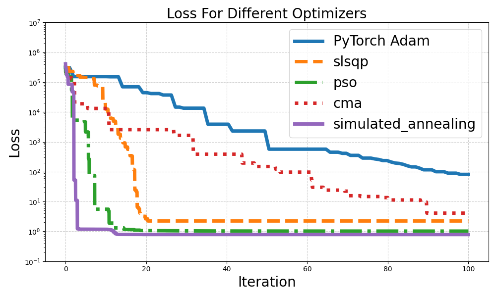
What do we see here?
Well, even though we tried to optimize the Adam learning rate as much as possible, all the other optimizers beat it. Specifically, the simulated annealing SA optimizer ran the fastest, reaching a loss value less than 100 it in only 2 iterations compared to 100 for Adam, a 50X improvement!
That said, take this with a grain of salt since every “iteration” of the SA requires many objective evaluations, each only requiring a forward pass. So, the “iterations” aren’t totally comparable.
CMA-ES ran the slowest, but that’s forgivable since it is designed for the hardest problems in the world, not just to converge fast. Lastly,PSO and SLSQP and also performed really well, coming in second and third places, respectfully.
Conclusion
So, Which One Should You Use?
Well, it depends.
If you can find a set of 100–1000 parameters (or hyperparameters) that you are having a hard time optimizing or that use non-differentiable operations — I would definitely recommend trying at least one of these optimizers.
Actually, just try them regardless!
Even if you can optimize your parameters with Adam or SGD, I’d recommend trying these approaches; you’d be surprised at how well they can perform since they may converge to much better local minima than your traditional gradient-based approaches can reach.
Sources and Further Reading:
[1] N. Hansen, The CMA evolution strategy: A tutorial (2016), arXiv preprint arXiv:1604.00772.
[2] J. Kennedy and R. Eberhart, Particle swarm optimization (1995), Proceedings of ICNN’95 — International Conference on Neural Networks, vol. 4, pp. 1942–1948.
[3] J. Nocedal and S. J. Wright, Numerical Optimization (1999),New York, NY: Springer New York.
[4] C. Tsallis and D. A. Stariolo, Generalized simulated annealing (1996), Physica A: Statistical Mechanics and its Applications, vol. 233, no. 1–2, pp. 395–406.
[5] Kingma, Diederik P. Adam: A method for stochastic optimization (2014), arXiv preprint arXiv:1412.6980.
[6] S. Ruder, An overview of gradient descent optimization algorithms (2016), arXiv preprint arXiv:1609.04747.
PyTorch Optimizers Aren’t Fast Enough. Try These Instead was originally published in Towards Data Science on Medium, where people are continuing the conversation by highlighting and responding to this story.
from Datascience in Towards Data Science on Medium https://ift.tt/MoAtQxy
via IFTTT


