Datascience in Towards Data Science on Medium,

Support Vector Classifier, Explained: A Visual Guide with Mini 2D Dataset

10/01/2024 Jesus Santana

CLASSIFICATION ALGORITHM

Finding the best “line” to separate the classes? Yeah, sure...

“Support Vector Machine (SVM) for classification works on a very basic principle — it tries to find the best line that separates the two classes.” But if I hear that oversimplified explanation one more time, I might just scream into a pillow.

While the premise sounds simple, SVM is one of those algorithms packed with mathematical gymnastics that took me an absurd amount of time to grasp. Why is it even called a ‘machine’? Why do we need support vectors? Why are some points suddenly not important? And why does it have to be a straight line — oh wait, a straight hyperplane??? Then there’s the optimization formula, which is apparently so tricky that we need another version called the dual form. But hold on, now we need another algorithm called SMO to solve that? What’s with all the dual coefficients that scikit-learn just spits out? And if that’s not enough, we’re suddenly pulling off this magic ‘kernel tricks’ when a straight line doesn’t cut it? Why do we even need these tricks? And why do none of the tutorials ever show the actual numbers?!

In this article, I’m trying to stop this Support Vector Madness. After hours and hours trying to really understand this algorithm, I will try to explain what’s ACTUALLY going on with ACTUAL numbers (and of course, its visualization too) but without the complicated maths, perfect for beginners.

Definition

Support Vector Machines are supervised learning models used mainly for classification tasks, though they can be adapted for regression as well. SVMs aim to find the line that best divides a dataset into classes (sigh…), maximizing the margin between these classes.

“Support vectors” are the data points that lie closest to the line and can actually define that line as well. And, what’s with the “Machine” then ? While other machine learning algorithms could include “Machine,” SVM’s naming may be partly due to historical context when it was developed. That’s it.

📊 Dataset Used

To understand how SVM works, it is a good idea to start from a dataset with few samples and smaller dimension. We’ll use this simple mini 2D dataset (inspired by [1]) as an example.

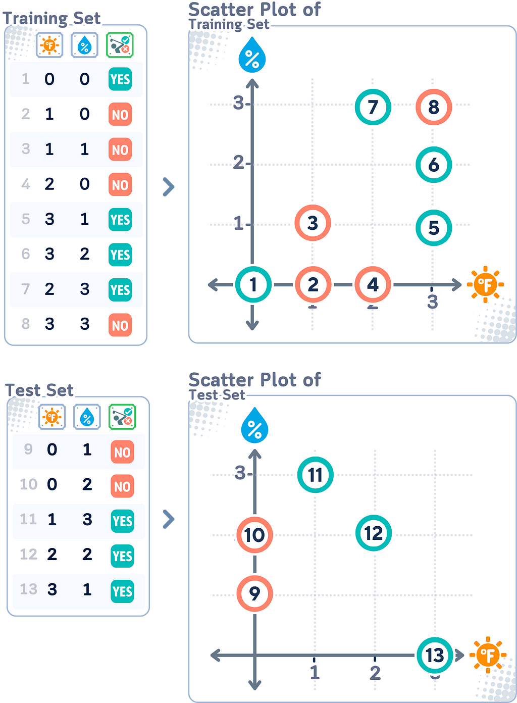
Instead of explaining the steps of the training process itself, we will walk from keyword to keyword and see how SVM actually works:

Part 1: Basic Components

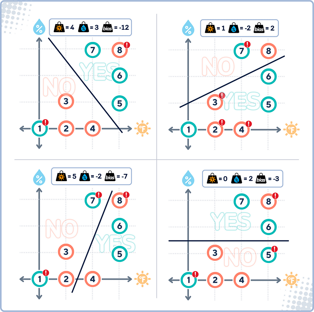
Decision Boundary

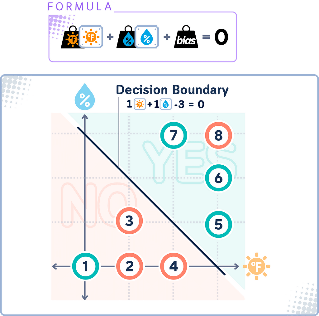
The decision boundary in SVM is the line (or called “hyperplane” in higher dimensions) that the algorithm determines to best separate different classes of data.

This line would attempt to keep most “YES” points on one side and most “NO” points on the other. However, because for data that isn’t linearly separable, this boundary won’t be perfect — some points might be on the “wrong” side.

Once this line is established, any new data can be classified depending on which side of the boundary it falls.

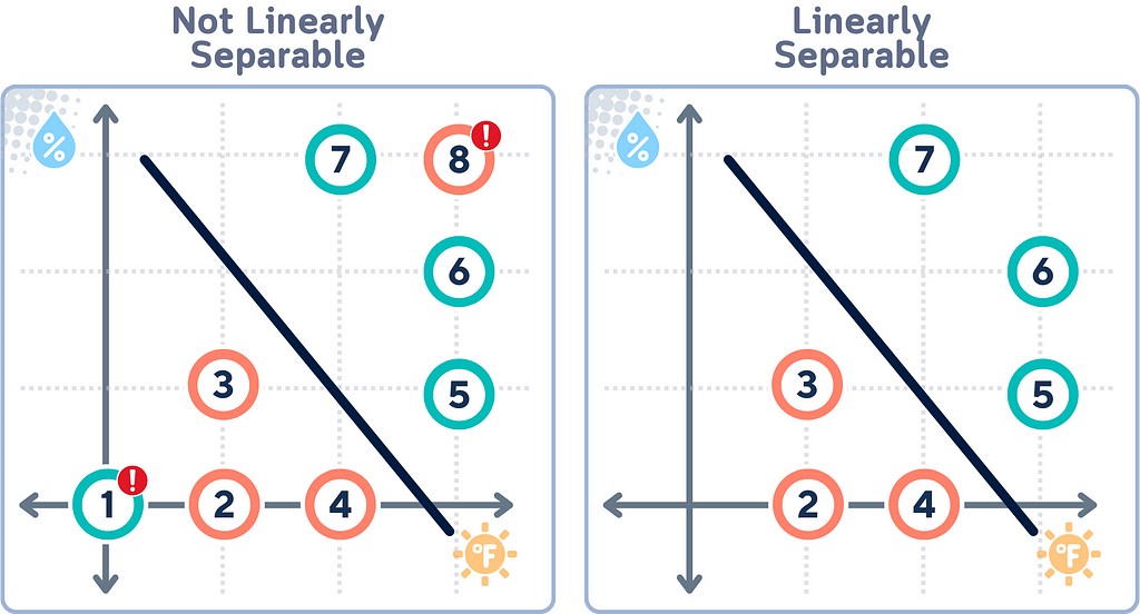
Linear Separability

Linear separability refers to whether we can draw a straight line that perfectly separates two classes of data points. If data is linearly separable, SVM can find a clear, hard boundary between classes. However, when data isn’t linearly separable (as in our case) SVM needs to use more advanced techniques.

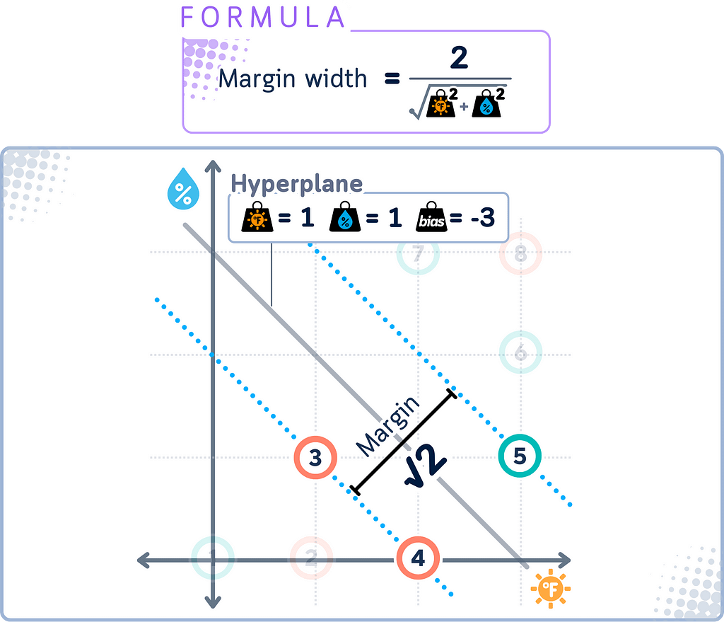
Margin

The margin in SVM is the distance between the decision boundary and the closest data points from each class. These closest points are called support vectors.

SVM aims to maximize this margin. A larger margin generally leads to better generalization — the ability to correctly classify new, unseen data points.

However, because data in general isn’t perfectly separable, SVM might use a soft margin approach. This allows some points to be within the margin or even on the wrong side of the boundary, trading off perfect separation for a more robust overall classifier.

Hard Margin vs Soft Margin

Hard Margin SVM is the ideal scenario where all data points can be perfectly separated by the decision boundary, with no misclassifications. In this case, the margin is “hard” because it doesn’t allow any data points to be on the wrong side of the boundary or within the margin.

Soft Margin SVM, on the other hand, allows some flexibility. It permits some data points to be misclassified or to lie within the margin. This allows the SVM to find a good balance between:

1. Maximizing the margin
2. Minimizing classification errors

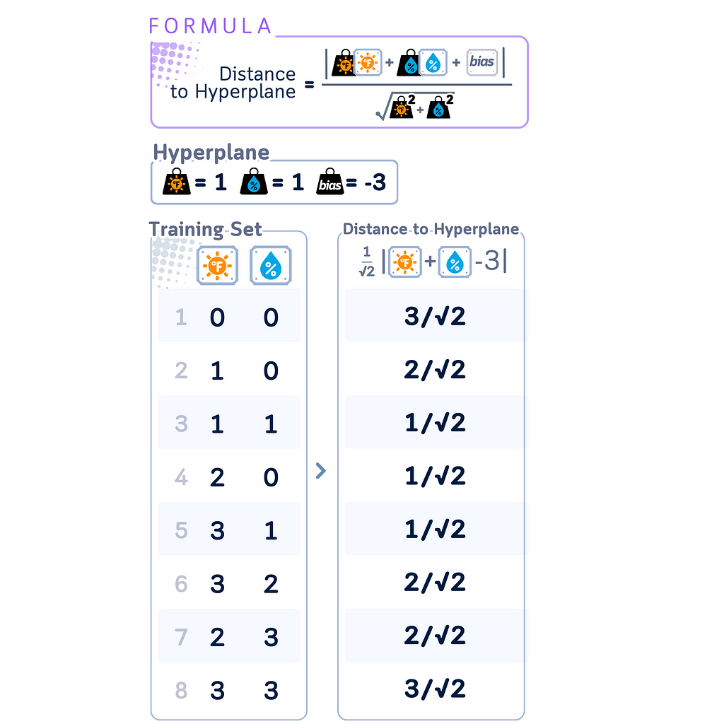
Distance Calculation

In SVM, distance calculations play an important role in both training and classification. The distance of a point x from the decision boundary is given by:

|w · x + b| / ||w||

where w is the weight vector perpendicular to the hyperplane, b is the bias term, and ||w|| is the Euclidean norm of w.

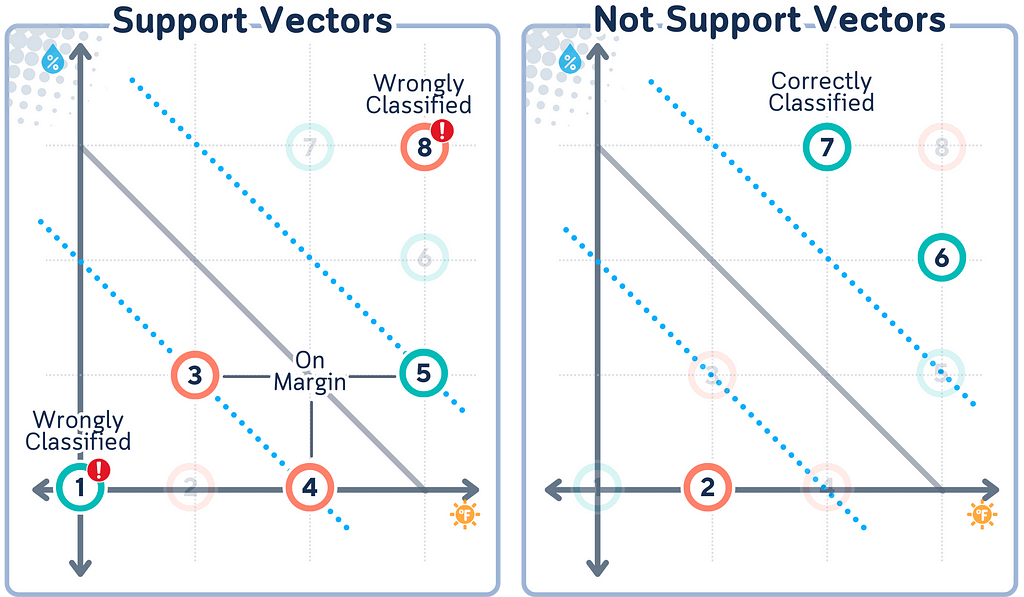
Support Vectors

Support vectors are the data points with closest distance to the hyperplane. They are important because: They “support” the hyperplane, defining its position.

What makes Support Vectors special is that they are the only points that matter for determining the decision boundary. All other points could be removed without changing the boundary’s position. This is a key feature of SVM — it bases its decision on the most critical points rather than all data points.

Slack Variables

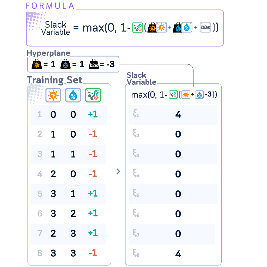
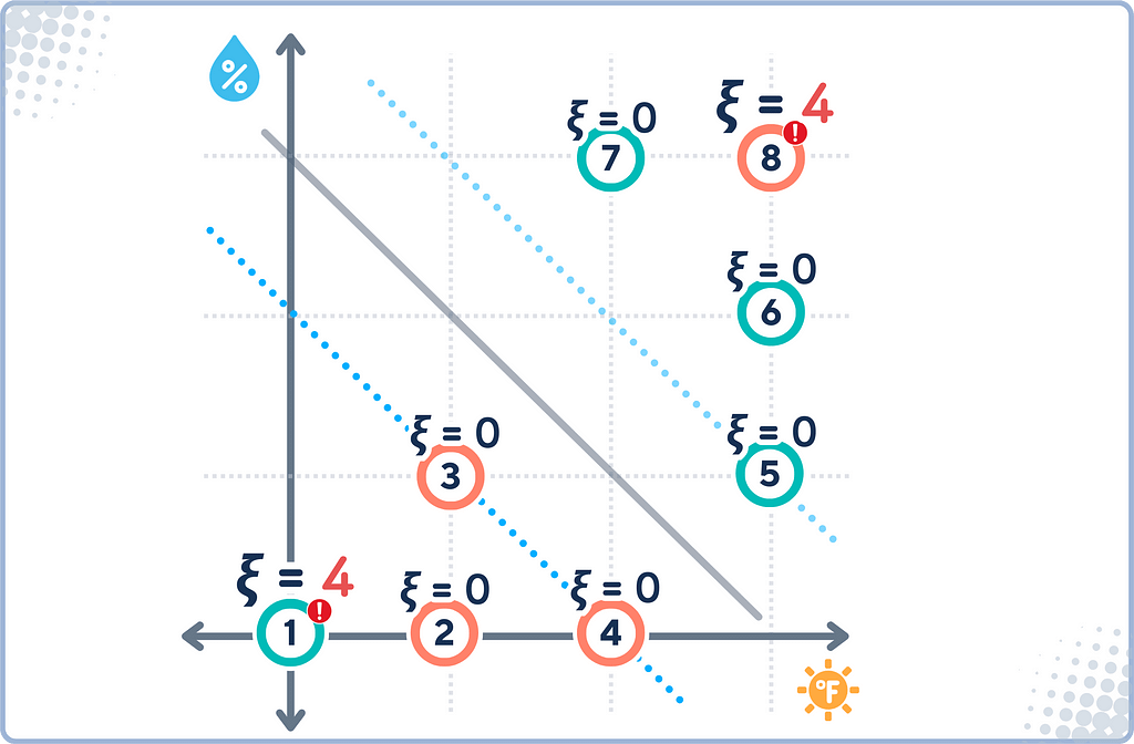
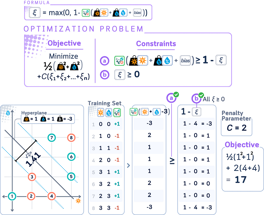
Slack Variables are introduced in Soft Margin SVM to quantify the degree of misclassification or margin violation for each data point. They’re called “slack” because they give the model some slack or flexibility in fitting the data.

In SVMs, slack variables ξᵢ can be calculated as:

ξᵢ = max(0, 1 — yᵢ(w · xᵢ + b))

where
· w is the weight vector
· b is the bias term
· xᵢ are the input vectors
· yᵢ are the corresponding labels

This formula only works when class labels yᵢ are in {-1, +1} format. It elegantly handles both classes:
· Correctly classified points beyond margin: ξᵢ = 0
· Misclassified or margin-violating points: ξᵢ > 0

Using {-1, +1} labels maintains SVM’s mathematical symmetry and simplifies optimization, unlike {0, 1} labels which would require separate cases for each class.

Primal Form for Hard Margin

The primal form is the original optimization problem formulation for SVMs. It directly expresses the goal of finding the maximum margin hyperplane in the feature space.

In simple terms, the primal form seeks to:

1. Find a hyperplane that correctly classifies all data points.
2. Maximize the distance between this hyperplane and the nearest data points from each class.

Primal form is:

minimize: (1/2) ||w||²
subject to: yᵢ(w · xᵢ + b) ≥ 1 for all i

where
· w is the weight vector
· b is the bias term
· xᵢ are the input vectors
· yᵢ are the corresponding labels (+1 or -1)
· ||w||² is the squared Euclidean norm of w

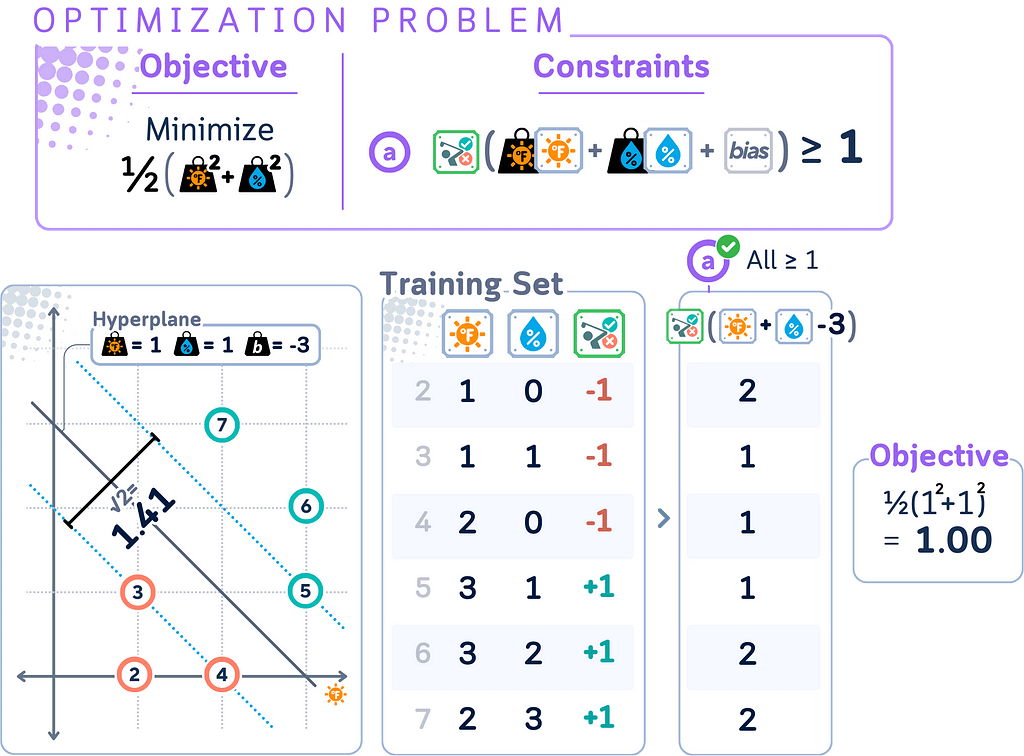
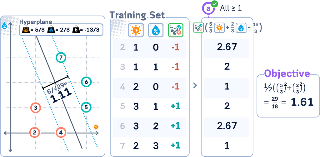
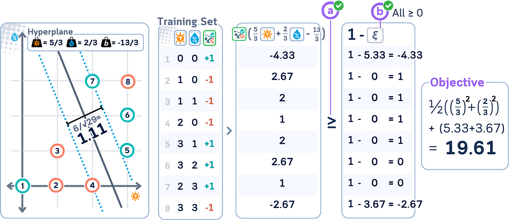
Primal Form for Soft Margin

Remember that the soft margin SVM is an extension of the original (hard margin) SVM that allows for some misclassification? This change is reflected in the primal form. The soft margin SVM primal form becomes:

minimize: (1/2) ||w||² + C Σᵢ ξᵢ
subject to: yᵢ(w · xᵢ + b) ≥ 1 — ξᵢ for all i, ξᵢ ≥ 0 for all i

where
· C is the penalty parameter
· ξᵢ are the slack variables
· All other variables are the same as in the hard margin case

Dual Form

Here’s the bad news: The primal form can be slow and hard to solve, especially for complex data.

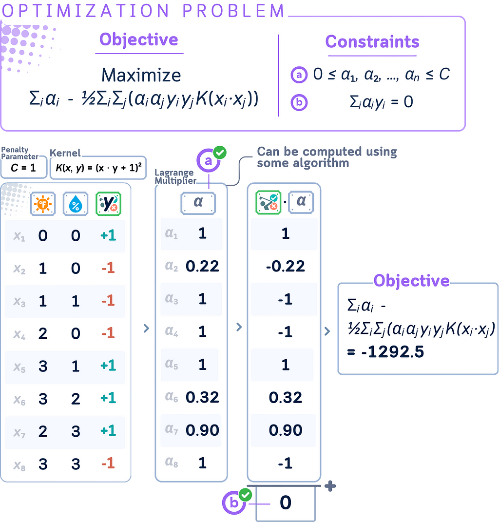
The dual form provides an alternative way to solve the SVM optimization problem, often leading to computational advantages. It’s formulated as follows:

maximize: Σᵢ,ⱼ(αᵢyᵢ) - ½ΣᵢΣⱼ(αᵢαⱼyᵢyⱼ(xᵢ · xⱼ))
subject to: 0 ≤ αᵢ ≤ C for all i, Σᵢαᵢyᵢ = 0

Where:
· αᵢ are the Lagrange multipliers (dual variables)
· yᵢ are the class labels (+1 or -1)
· xᵢ are the input vectors
· C is the regularization parameter (upper bound for αᵢ)
· (xᵢ · xⱼ) denotes the dot product between xᵢ and xⱼ

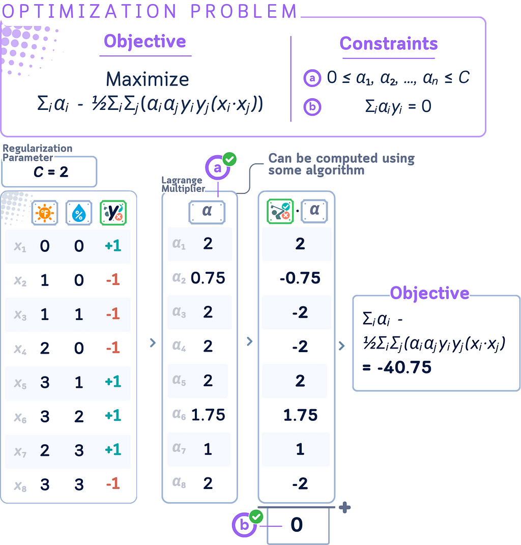
Lagrange Multipliers

As we notice in the dual form, Lagrange multipliers (αᵢ) show up when we transform the primal problem into its dual form (that’s why they also known as the dual coefficients). If you noticed, the weights & bias are no longer there!

Each data point in the training set has an associated Lagrange multiplier. The good thing is Lagrange multipliers make things much easier to understand:

1. Interpretation:
   - αᵢ = 0: The point is correctly classified and outside the margin. This point does not influence the decision boundary.
   - 0 < αᵢ < C: The point is on the margin boundary. These are called “free” or “unbounded” support vectors.
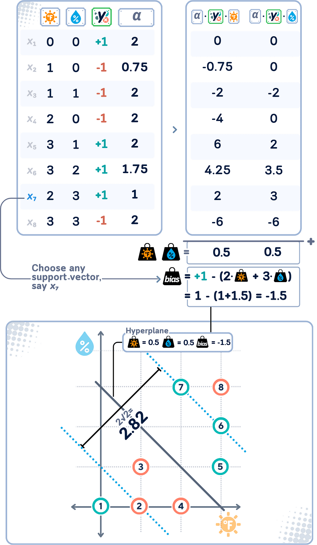
   - αᵢ = C: The point is either on or inside the margin (including misclassified points). These are called “bound” support vectors.
2. Relationship to decision boundary:
   w = Σᵢ(αᵢ yᵢ xᵢ),
   b = yᵢ — Σⱼ(αᵢ yⱼ(xⱼ · xᵢ))
   where yᵢ is the label of any (unbounded) support vector.
   This means the final decision boundary is determined only by points with non-zero αᵢ !

Sequential Minimal Optimization

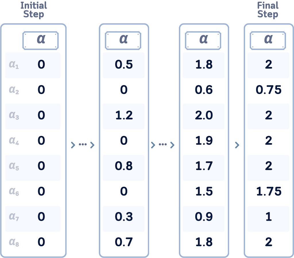
Remember that we haven’t really shown how to get the optimal Lagrange multipliers (αᵢ)? The algorithm to solve this is called Sequential Minimal Optimization (SMO). Here’s a simplified view of how we get these values:

1. Start with all αᵢ at zero.
2. Repeatedly select and adjust two αᵢ at a time to improve the solution.
3. Update these pairs quickly using simple math.
4. Ensure all updates follow SVM constraints.
5. Repeat until all αᵢ are “good enough.”
6. Points with αᵢ > 0 become support vectors.

This approach efficiently solves the SVM optimization without heavy computations, making it practical for large datasets.

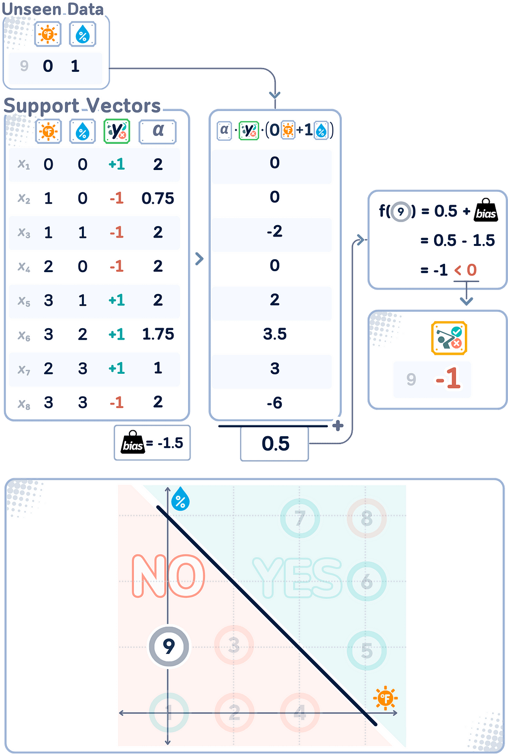
Decision Function

After solving the SVM optimization problem using the dual form and obtaining the Lagrange multipliers, we can define the decision function. This function determines how new, unseen data points are classified by the trained SVM model.

f(x) = Σᵢ(αᵢyᵢ(xᵢ · x)) + b

Here, αᵢ are the Lagrange multipliers, yᵢ are the class labels (+1 or -1), xᵢ are the support vectors, and x is the input vector to be classified. The final classification for a new point x is determined by the sign of f(x) (either “+” or “-”).

Note that this decision function uses only the support vectors (data points with non-zero αᵢ) to classify new inputs, which is the core principle of the SVM algorithm!

🌟 Support Vector Classifier Code

The results above can be obtained using the following code:

import numpy as np
import pandas as pd
from sklearn.svm import SVC

# Create DataFrame
df = pd.DataFrame({
    '🌞': [0, 1, 1, 2, 3, 3, 2, 3, 0, 0, 1, 2, 3],
    '💧': [0, 0, 1, 0, 1, 2, 3, 3, 1, 2, 3, 2, 1],
    'y': [1, -1, -1, -1, 1, 1, 1, -1, -1, -1, 1, 1, 1]
}, index=range(1, 14))

# Split into train and test
train_df, test_df = df.iloc[:8].copy(), df.iloc[8:].copy()
X_train, y_train = train_df[['🌞', '💧']], train_df['y']
X_test, y_test = test_df[['🌞', '💧']], test_df['y']

# Create and fit SVC model
svc = SVC(kernel='linear', C=2)
svc.fit(X_train, y_train)

# Add Lagrange multipliers and support vector status
train_df['α'] = 0.0
train_df.loc[svc.support_ + 1, 'α'] = np.abs(svc.dual_coef_[0])
train_df['Is SV'] = train_df.index.isin(svc.support_ + 1)

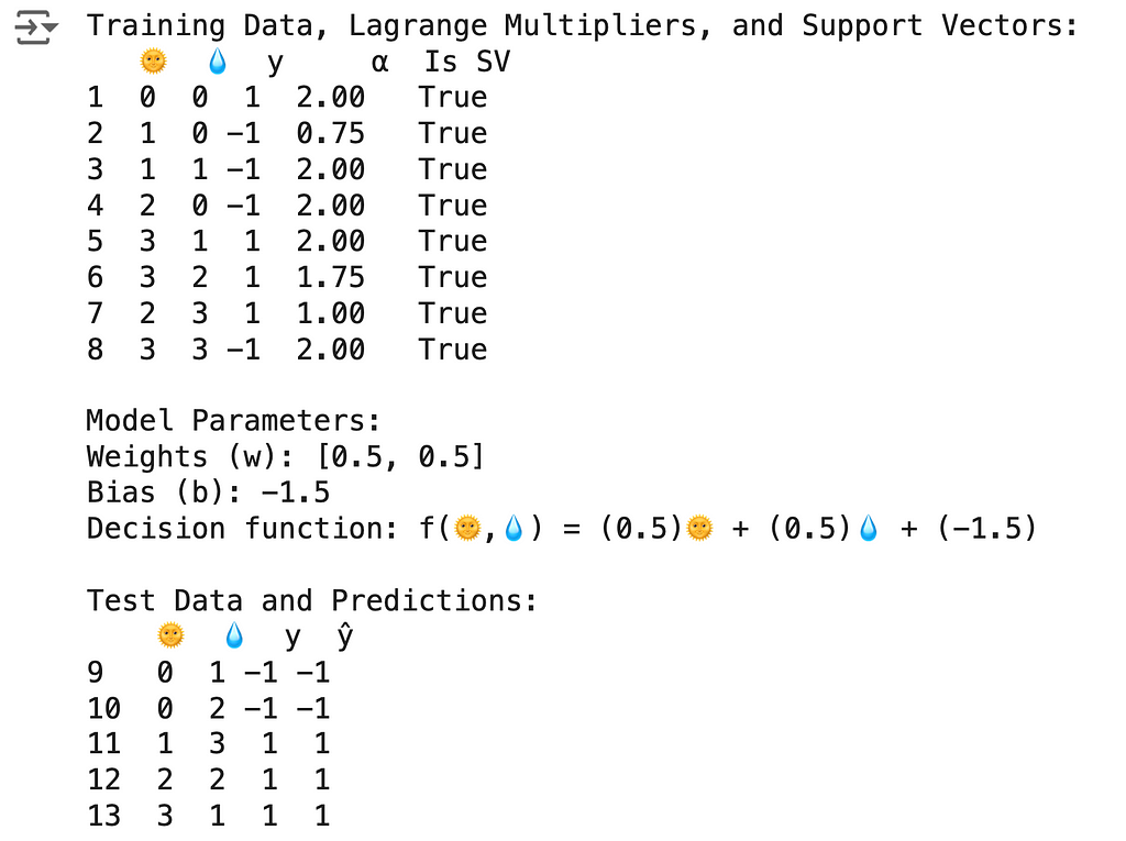
print("Training Data, Lagrange Multipliers, and Support Vectors:")
print(train_df)

# Print model parameters
w, b = svc.coef_[0], svc.intercept_[0]
print(f"\nModel Parameters:")
print(f"Weights (w): [{w[0]}, {w[1]}]")
print(f"Bias (b): {b}")
print(f"Decision function: f(🌞,💧) = ({w[0]})🌞 + ({w[1]})💧 + ({b})")

# Make predictions
test_df['ŷ'] = svc.predict(X_test)

print("\nTest Data and Predictions:")
print(test_df)

Part 2: Kernel Trick

As we have seen so far, no matter how we set up the hyperplane, we never could make a perfect separation between the two classes. There are actually some “trick” that we can do to make it separable… even though it is not linearly anymore.

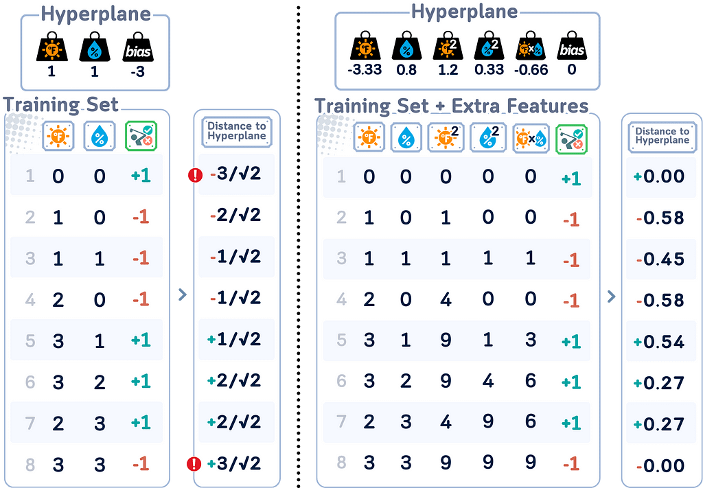
Input Space vs Feature Space

Input Space refers to the original space of your data features. In our golf dataset, the Input Space is two-dimensional, consisting of temperature and humidity. Each data point in this space represents a specific weather condition where someone decided to play golf or not.

Feature Space, on the other hand, is a transformed version of the Input Space where the SVM actually performs the classification. Sometimes, data that isn’t linearly separable in the Input Space becomes separable when mapped to a higher-dimensional Feature Space.

Kernel and Implicit Transformation

A kernel is a function that computes the similarity between two data points, implicitly representing them in a higher-dimensional space (the feature space).

Say, there’s a function φ(x) that transforms each input point x to a higher-dimensional space. For example: φ : ℝ² → ℝ³, φ(x,y) = (x, y, x² + y²)

Common Kernels and Their Implicit Transformations:
a. Linear Kernel: K(x,y) = x · y
- Transformation:
φ(x) = x (identity)
- This doesn’t actually change the space but is useful for linearly separable data.

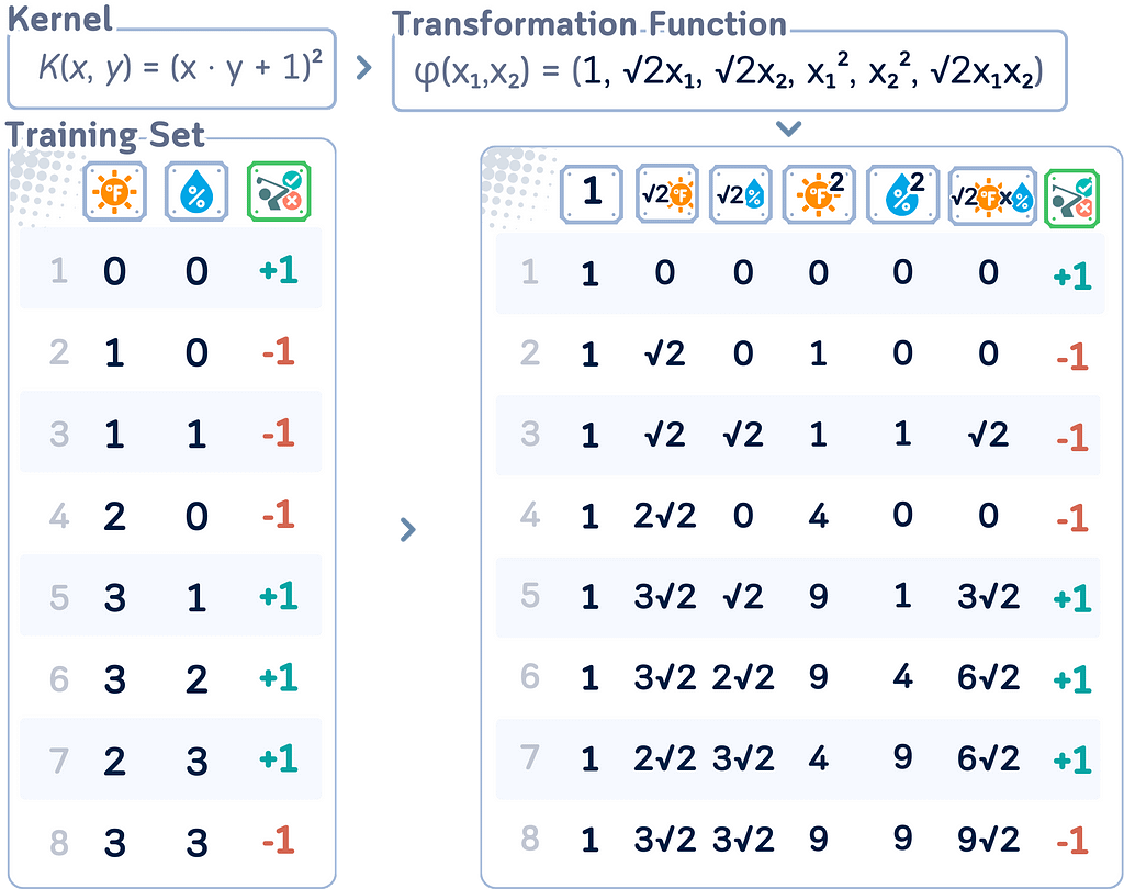
b. Polynomial Kernel: K(x,y) = (x · y + c)ᵈ
- Transformation (for d = 2, c = 1 in ℝ²):
φ(x₁,x₂) = (1, √2x₁, √2x₂, x₁², √2x₁x₂, x₂²)
- This captures all polynomial terms up to degree d.

c. RBF Kernel: K(x,y) = exp(-γ||x - y||²)
- Transformation (as an infinite series):
φ(x₁,x₂)= exp(-γ||x||²) * (1, √(2γ)x₁, √(2γ)x₂, …, √(2γ²/2!)x₁², √(2γ²/2!)x₁x₂, √(2γ²/2!)x₂², …, √(2γⁿ/n!)x₁ⁿ, …)
- Can be thought of as a similarity measure that decreases with distance.

Kernel Trick

The “trick” part of the kernel trick is that we can perform operations in this higher-dimensional space solely using the kernel function, without ever explicitly computing the transformation φ(x).

Notice that in the dual form, the data points only appear as dot products (xᵢ · xⱼ). This is where the kernel trick comes in. We can replace this dot product with a kernel function: (xᵢ · xⱼ) → K(xᵢ, xⱼ)

This process cannot be done if we are just using the primal form, that is one of the main reason why the dual form is preferable!

This substitution implicitly maps the data to a higher-dimensional space without explicitly computing the transformation.

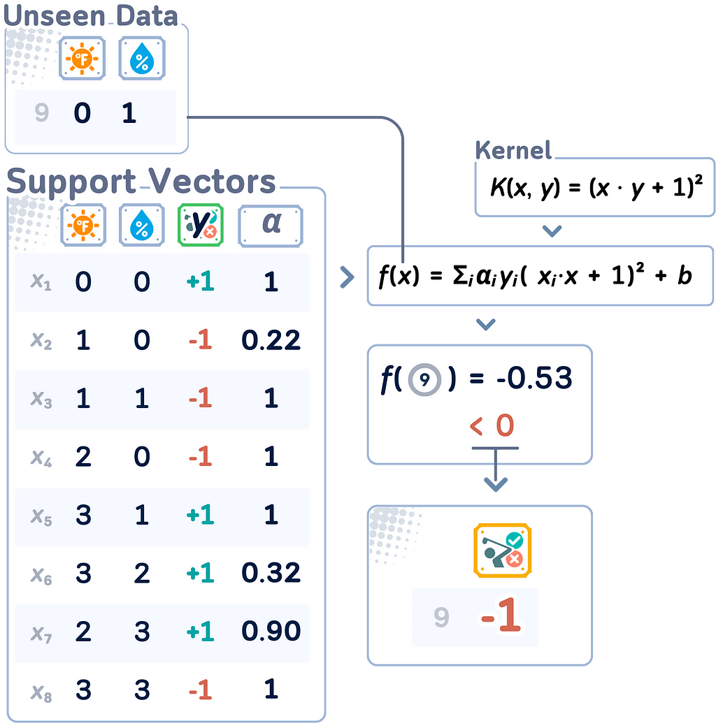
Decision Function with Kernel Trick

The resulting decision function for a new point x becomes:

f (x) = sign(Σᵢ αᵢyᵢK(xᵢ, x) + b)

where the sum is over all support vectors (points with αᵢ > 0).

🌟 Support Vector Classifier (with Kernel Trick) Code Summary

The results above can be obtained using the following code:

import numpy as np
import pandas as pd
from sklearn.svm import SVC

# Create DataFrame
df = pd.DataFrame({
    '🌞': [0, 1, 1, 2, 3, 3, 2, 3, 0, 0, 1, 2, 3],
    '💧': [0, 0, 1, 0, 1, 2, 3, 3, 1, 2, 3, 2, 1],
    'y': [1, -1, -1, -1, 1, 1, 1, -1, -1, -1, 1, 1, 1]
}, index=range(1, 14))

# Split into train and test
train_df, test_df = df.iloc[:8].copy(), df.iloc[8:].copy()
X_train, y_train = train_df[['🌞', '💧']], train_df['y']
X_test, y_test = test_df[['🌞', '💧']], test_df['y']

# Create and fit SVC model with polynomial kernel
svc = SVC(kernel='poly', degree=2, coef0=1, C=1)
svc.fit(X_train, y_train)

# Add Lagrange multipliers and support vector status
train_df['α'] = 0.0
train_df.loc[svc.support_ + 1, 'α'] = np.abs(svc.dual_coef_[0])
train_df['Is SV'] = train_df.index.isin(svc.support_ + 1)

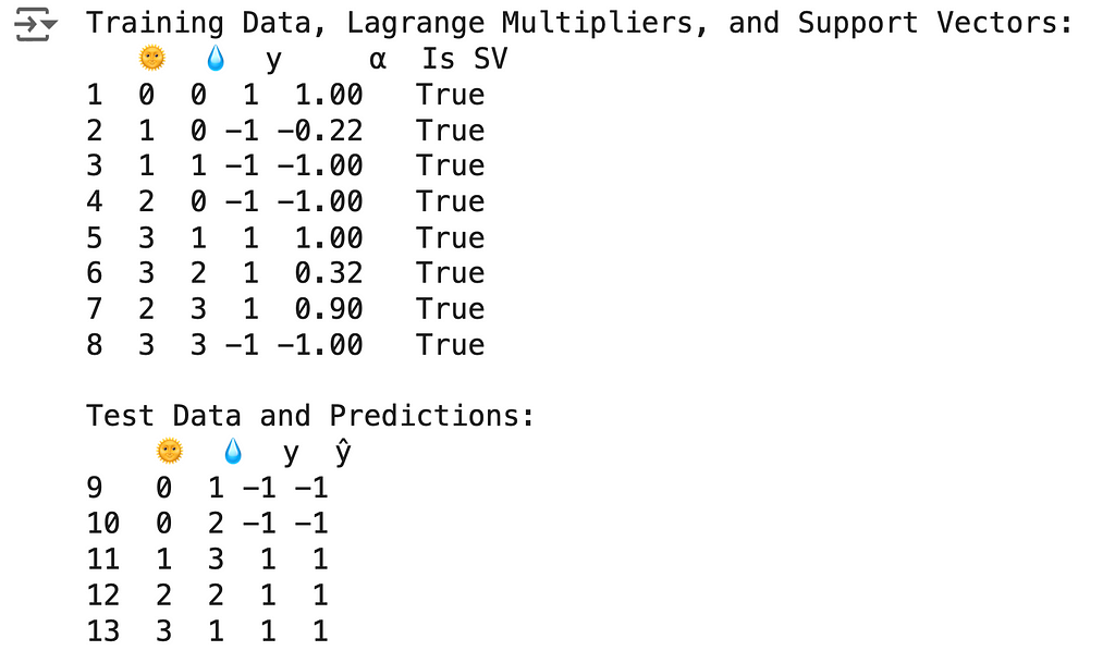
print("Training Data, Lagrange Multipliers, and Support Vectors:")
print(train_df)

# Make predictions
test_df['ŷ'] = svc.predict(X_test)
print("\nTest Data and Predictions:")
print(test_df)

Key Parameters

In SVM, the key parameter would be the penalty/regularization parameter C:

• Large C: Tries hard to classify all training points correctly, potentially overfitting
• Small C: Allows more misclassifications but aims for a simpler, more general model

Of course, if you are using non-linear kernel, you also need to adjust the degree (and coefficients) related to that kernel.

Final Remarks

We’ve gone over a lot of the key concepts in SVMs (and how they work), but the main idea is this: It’s all about finding the right balance. You want your SVM to learn the important patterns in your data without trying too hard on getting every single training data on the correct side of the hyperplane. If it’s too strict, it might miss the big picture. If it’s too flexible, it might see patterns that aren’t really there. The trick is to tune your SVM so it can identify the real trends while still being adaptable enough to handle new data. Get this balance right, and you’ve got a powerful tool that can handle all sorts of classification problems.

Further Reading

For a detailed explanation of the Support Vector Machine and its implementation in scikit-learn, readers can refer to the official documentation [2], which provides comprehensive information on its usage and parameters.

Technical Environment

This article uses Python 3.7 and scikit-learn 1.5. While the concepts discussed are generally applicable, specific code implementations may vary slightly with different versions.

About the Illustrations

Unless otherwise noted, all images are created by the author, incorporating licensed design elements from Canva Pro.

Reference

[1] T. M. Mitchell, Machine Learning (1997), McGraw-Hill Science/Engineering/Math, pp. 59

[2] F. Pedregosa et al., Scikit-learn: Machine Learning in Python, Journal of Machine Learning Research, vol. 12, pp. 2825–2830, 2011. [Online]. Available: https://scikit-learn.org/stable/modules/generated/sklearn.svm.SVC.html

---

Support Vector Classifier, Explained: A Visual Guide with Mini 2D Dataset was originally published in Towards Data Science on Medium, where people are continuing the conversation by highlighting and responding to this story.

from Datascience in Towards Data Science on Medium https://ift.tt/6QTYgPu
via IFTTT