Techniques for Chat Data Analytics with Python
Part I: Communication Density Analysis

and obtained from Pexels.com
For many years now, our communication has become increasingly digital. Whether through quick text messages via chat applications or sending emails, digital messaging has firmly embedded itself in our daily lives.
This leads to an increase in the amount of digitally produced data.
Since communication involves at least two individuals, it can reveal a lot of insights about the participants and their relationship with each other.
This article will be the first part of a series where I will show you the cool things you can do with your chats and the personal insights you can gain from them. You can always find the Python code and any Tableau files I create for visualizations on my GitHub profile.
The Goal
Since this is the first article of the series, I would like to start with a high-level analysis of the metadata from WhatsApp chats. I have named the upcoming analysis Communication Density Analysis because the main feature of the visualization emerges from the density of the sent messages.

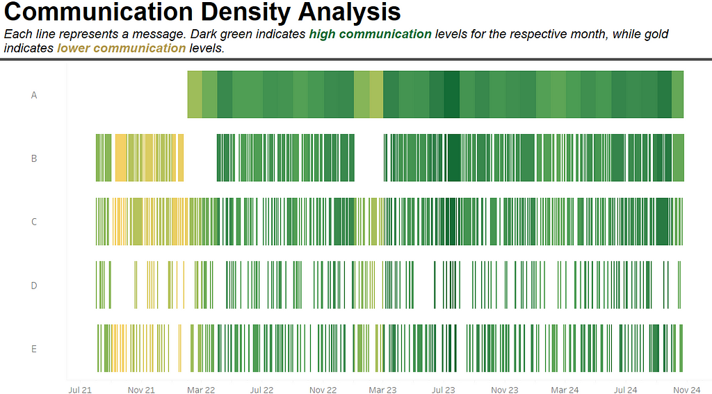
This event plot shows the communication between an artificially created person, let’s call him John, and five of his closest chat partners, whom we will initially refer to as A, B, C, D, and E. Later, I will reveal the identities of these five individuals and explain the relationships John has with each of them.
In the event plot, each line represents a message. The different rows display the respective chats. The darker the green, the more messages have been exchanged between the individuals in the chat. If the lines turn golden, it indicates that there was communication, but only a few messages were sent.
The interesting aspect of this type of analysis is that it can provide insights into the person whose chats you are examining. For example, we see that the chat with Person A only started around February 2022 and quickly became quite intensive. There are no gaps or whitespace in this chat, so we can assume there is intensive daily communication. Could it be that John started dating someone who has become a very special person in his life?
Not only can you gain insights into who might be someone’s potential girlfriend or boyfriend and identify when people meet, but you can also detect conflicts between individuals. For instance, Person B regularly communicated with John, but the intensity decreased until February 2022, when suddenly the digital contact ceased. Could it be that John was involved in a serious conflict with Person B around this time? Perhaps it’s just a coincidence that he started to communicate more intensively with Person A during this period — was the conflict perhaps related to Person A? Of course, there could be many explanations for gaps in communication, but we can definitely see that something happened in the data, and possible relationships can be identified.
However, about a year later, John and Person B experienced another communication gap, followed by intensive and frequent communication. Person C seems to have always engaged in frequent and high-intensity communication, which has also increased over time. There are some gaps in their communication, suggesting that it may not be daily but rather regular and frequent — perhaps resembling communication with a best friend.
Persons D and E exhibit a similar pattern regarding the intensity of communication with John. When they do communicate, they tend to send more messages. However, communication with Person D appears to happen less frequently, although both could be good friends or family members.
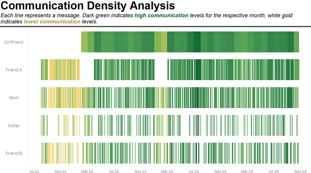
Now that we’ve examined the data, let’s unveil the identities of the individuals hiding behind A, B, C, D, and E:

Indeed, Person A was actually John’s girlfriend, whom he met for the first time in February 2022. Person B was his best friend, with whom he lost contact after spending more time with his new girlfriend and rebuilding their relationship. Around February 2023, they had a fight and lost contact again for a while. It seems that John communicates regularly with his mom but has less frequent communication with his sister. Finally, Person E was his old school friend, with whom there are sometimes communication gaps, but they always find their way back to each other.
Now that you’ve seen the insights you can generate, I recommend trying it with your own messages. I tested this with some of my WhatsApp chats, and it is fascinating to see what emerges from the analysis. To make it easier for you, I will now show you how to create the visualization with your own data.
How to create the event plot?
The first step is of course to get the data. I personally did it with Whatsapp. For that you can find here an easy and fast instruction how to get your data. If you have downloaded it you get text files that could look like this
16.01.24, 15:13 - John Snow is a contact.
16.01.24, 15:13 - John Snow: <Media Excluded>
16.01.24, 15:13 - John Snow: Hi! How are you?😀
16.01.24, 15:16 - Maria: Hey, I’m doing well, thanks! How about you?
16.01.24, 15:17 - John Snow: I’m good too, just been busy with work lately.
16.01.24, 15:19 - Maria: I can relate! Anything exciting going on?
16.01.24, 15:21 - John Snow: Not much, just trying to catch up with everything. What about you?
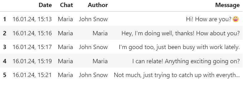
To create an event plot, we need to extract the messages, the date, the author, and the chat to generate the visualization. As you can see, there are also texts saved that say “X is a contact” or “<Media Excluded>”. We will need to filter out these rows in the future. Note that since your messenger may be set to a different language, it might use different expressions that also need to be filtered out. I will explain where in the upcoming code you can enter your expressions if needed. But first, let’s check the table structure to see how it should look to create the event plot.

We have the Date column, which includes the hours and minutes when the message was sent. In our example, we are chatting in the Maria chat, and the authors are John and Maria. If you apply this to groups, there may be more than two authors. In the Message column, the messages will be collected, which enables incredible analysis possibilities. However, those will be explored in the upcoming parts of this series.
To start with the transformation and move from the text files to a structured format, we first need to load the data.
import pandas as pd
import glob
import os

folder_path = r"C:\Users\Robin\Whatsapp_chats"  #Enter your folderpath Folder path here

# Returns a list with all file_paths in the folder with .txt ending
all_files = glob.glob(os.path.join(folder_path, "*.txt"))

# Create empty list for DataFrames
dfs = []
Therefore we start by importing the nececarry libraries and we define the folder path, where our chats are safed in text files. Then we would like to have a list with all file paths to the respective chats in the folder that contain the txt endings. Therefore we create the all_files variable. In the third step we create an empty list for the dataframes that we will collect.
# Read all filed, add the file name as column and append these to the list dfs
for file in all_files:
    df = pd.read_csv(file, sep='\t', engine='python', header=None, names=['Text'], on_bad_lines='warn', encoding='utf-8')
    df['Filename'] = os.path.basename(file)  # Dateiname hinzufügen
    dfs.append(df)

# Combine all DataFrames with the concat command.
chat = pd.concat(dfs, ignore_index=True)
Now that we have loaded all the chat data into one DataFrame, there are two more things to do:
- Filter out rows that do not include messages.
- Split the data into Date, Chat, Author, and Message columns.
For filtering, we will use a simple regex, a string match function, and a specific string contains function.
# Define Pattern for Message rows
pattern = r'\d{2}\.\d{2}\.\d{2}, \d{2}:\d{2} - .+: .*'

# Filter the rows
chat = chat[chat['Text'].str.match(pattern)]
chat = chat[~chat['Text'].str.contains(r'(<Media Excluded>|null)')]
The first filter excludes all rows that do not match the pattern defined by the regex. This way, we eliminate lines like “John Snow is a contact.”
The second filter removes all rows that contain expressions such as “null” or “<Media Excluded>.” In fact, all messages that are voice messages will be replaced with “null.” I find these messages uninteresting, but if you are interested in them, you can simply remove the “null” expression from the filter. If there are other rows that you would like to exclude, please add them to the str.contains expression.
In the second step, we only need to split the columns. To do this, we will use some split operations and then filter to the columns of interest.
# Extract Date
chat['Date'] = chat['Text'].str.split(' - ').str[0]

# Extract Author
chat['Author']=  chat.apply(lambda row: row['Text'].replace(row['Date'] + ' - ', ''), axis=1)

# Extract Chat - Adjust "WhatsApp-Chat mit " with your filename pattern
chat['Chat'] = chat['Filename'].str.replace('WhatsApp-Chat mit ', '').str.replace('.txt', '')

# Split Author column to Author and Message
chat[['Author', 'Message']] = chat['Author'].str.split(': ', n=1, expand=True)

# Filter relevant columns
chat = chat[['Date','Author','Message','Chat']]
One point I would like to mention here: When I extract my WhatsApp chats, the filename is saved with a German pattern. In my case, it is “WhatsApp-Chat mit Maria.txt”. To create the Chat column, I simply extracted the filename as an extra column and removed the left and right parts of “Maria.” You will likely need to adjust this based on your language.
After this, you will have your chats in a tabular form. You only need to download my Tableau file from my GitHub profile, edit the data source, and replace it with yours.
In my other article, The Transparent Human, I already demonstrated how dangerous specific data can be when used to answer personal questions about an individual, potentially leading to manipulation. If you apply the techniques from this blog to analyze specific chats, please ensure you obtain the other person’s consent, as this analysis can reveal insights they may not want you to know. In this way, we must respect the privacy of others.
Conclusion
In this first part of our series, we have explored the fascinating world of WhatsApp chat analysis, highlighting how even the metadata can reveal significant insights about interpersonal relationships. By examining communication density and patterns, we can uncover dynamics such as the emergence of new connections, potential conflicts, and the ebb and flow of friendships over time.
As you embark on your own journey of chat analysis, I encourage you to approach it with curiosity and responsibility. Download the provided Tableau file, apply the techniques discussed, and see what stories your chats tell.
Thanks for sticking around to the end! If you enjoyed this wild ride through chat analysis, give a clap or hit that follow button — your support keeps me caffeinated and inspired! In the next article, I’ll dive deeper into topic extraction: What were you and your friends writing about the most? Get ready for some exciting insights! Until then, happy chatting!
Techniques for Chat Data Analytics with Python was originally published in Towards Data Science on Medium, where people are continuing the conversation by highlighting and responding to this story.
from Datascience in Towards Data Science on Medium https://ift.tt/X2BYOSJ
via IFTTT


