
Understanding KL Divergence, Entropy, and Related Concepts
Important concepts in information theory, machine learning, and statistics

Introduction
In Information Theory, Machine Learning, and Statistics, KL Divergence (Kullback-Leibler Divergence) is a fundamental concept that helps us quantify how two probability distributions differ. It’s often used to measure the amount of information lost when one probability distribution is used to approximate another. This article will explain KL Divergence and some of the other widely used divergences.
KL Divergence
KL Divergence, also known as relative entropy, is a way to measure the difference between two probability distributions, denoted as P and Q. It is often written as —


This equation compares the true distribution P with the approximation. distribution Q. Imagine you’re compressing data using an encoding system optimized for one distribution (distribution Q) but the actual data comes from a different distribution (distribution P). KL Divergence measures how inefficient your encoding will be. If Q is close to P, the KL Divergence will be small, meaning less information is lost in the approximation. If Q differs from P, the KL Divergence will be large, indicating significant information loss. In other words, KL Divergence tells you how many extra bits you need to encode data from P when using an encoding scheme designed for Q.
KL Divergence and Shannon’s Entropy
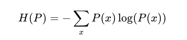
To better understand KL Divergence, it’s useful to relate it to entropy, which measures the uncertainty or randomness of a distribution. The Shannon’s Entropy of a distribution P is defined as:
Recall the popular Binary Cross Entropy Loss function and its curve. Entropy is a measure of uncertainty.

Entropy tells us how uncertain we are about the outcomes of a random variable. The lower the entropy, the more certain we are about the outcome. The lower the entropy, the more information we have. Entropy is the highest when p=0.5. A probability of 0.5 denotes maximum uncertainty. KL Divergence can be seen as the difference between the entropy of P and the “cross-entropy” between P and Q. Thus, KL Divergence measures the extra uncertainty introduced by using Q instead of P.

Properties —
- KL Divergence is always non-negative.

- Unlike other distance metrics, the KL Divergence is asymmetric.

Some Applications —
- In Variational Auto Encoders, KL Divergence is used as a regularizer to ensure that the latent variable distribution stays close to a prior distribution (typically a standard Gaussian).
- KL Divergence quantifies the inefficiency or information loss when using one probability distribution to compress data from another distribution. This is useful in designing and analyzing data compression algorithms.
- In reinforcement learning, KL Divergence controls how much a new policy can deviate from an old one during updates. For example, algorithms like Proximal Policy Optimization (PPO) use KL Divergence to constrain policy shifts.
- KL Divergence is widely used in industries to detect data drift.
Jensen-Shannon Divergence
Jensen-Shannon Divergence (JS Divergence) is a symmetric measure that quantifies the similarity between two probability distributions. It is based on the KL Divergence. Given two probability distributions P and Q, the Jensen-Shannon Divergence is defined as —
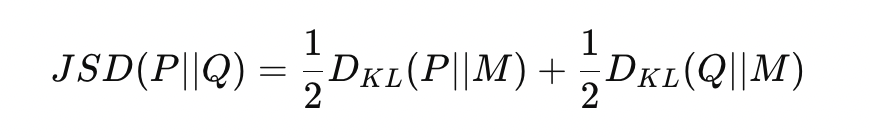
where M is the average (or mixture) distribution between P and Q.

The first term measures how much information is lost when M is used to approximate P. The second term measures the information loss when M is used to approximate Q. JS Divergence computes the average of the two KL divergences with respect to the average distribution M. KL Divergence penalizes you for using one distribution to approximate another. Still, it is sensitive to which distribution you start from. This asymmetry is often problematic when you want to compare distributions without bias. JS Divergence fixes this by averaging between the two distributions. It doesn’t treat either P or Q as the “correct” distribution but looks at their combined behavior through the mixture distribution M.
Renyi Entropy and Renyi Divergence
We saw earlier that KL Divergence is related to Shannon Entropy. Shannon Entropy is a special case of Renyi Entropy. Renyi Entropy of a distribution is defined as —

Renyi Entropy is parameterized by α>0. α controls how much weight is given to different probabilities in the distribution.
- α=1: Renyi Entropy equals Shannon Entropy, giving equal weightage to all probable events. You can derive it using limits and the L’Hospital rule.

- α<1: The entropy increases sensitivity to rare events (lower probabilities), making it more focused on the diversity or spread of the distribution.
- α>1: The entropy increases sensitivity to common events (higher probabilities), making it more focused on the concentration or dominance of a few outcomes.

- α=0: Renyi Entropy approaches the logarithm of the number of possible outcomes (assuming all outcomes are non-zero). This is called the Hartley Entropy.
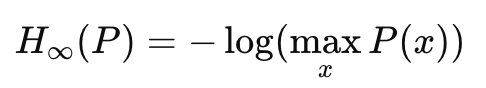
- α=∞: As α→∞, Renyi entropy becomes the min-entropy, focusing solely on the most probable outcome.
The Renyi Divergence is a metric based on Renyi Entropy. The Renyi Divergence between two distributions P and Q, parameterized by α is defined by —
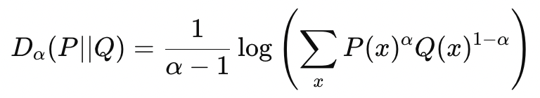
KL Divergence is a special case of Renyi Divergence, where α=1.

- α<1: Focuses on rare events; more sensitive to tail distributions.
- α>1: Focuses on common events; more sensitive to high-probability regions.
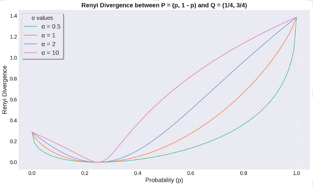
The Renyi Divergence is always non-zero and equal to 0 when P = Q. The above figure illustrates how the divergence changes when we vary the distribution P. The divergence increases, with the amount of increase depending on the value of α. A higher value α makes Renyi Divergence more sensitive to changes in probability distribution.
Renyi Divergence finds its application in Differential Privacy, an important concept in Privacy Preserving Machine Learning. Differential Privacy is a mathematical framework that guarantees individuals' privacy when their data is included in a dataset. It ensures that the output of an algorithm is not significantly affected by the inclusion or exclusion of any single individual’s data. Renyi Differential Privacy (RDP) is an extension of differential privacy that uses Rényi divergence to provide tighter privacy guarantees. We will discuss them in a future blog.
Toy Example — Detecting Data Drift
In an e-commerce setup, data drift can occur when the underlying probability distribution of user behavior changes over time. This can affect various aspects of the business, such as product recommendations. To illustrate how different divergences can be used to detect this drift, consider the following toy example involving customer purchase behavior over seven weeks.
Imagine an e-commerce platform that tracks customer purchases across five product categories: Electronics, Clothing, Books, Home & Kitchen, and Toys. The platform collects click data weekly on the proportion of clicks in each category. These are represented as probability distributions shown in the following code block.
weeks = {
    'Week 1': np.array([0.3, 0.4, 0.2, 0.05, 0.05]),
    'Week 2': np.array([0.25, 0.45, 0.2, 0.05, 0.05]),
    'Week 3': np.array([0.2, 0.5, 0.2, 0.05, 0.05]),
    'Week 4': np.array([0.15, 0.55, 0.2, 0.05, 0.05]),
    'Week 5': np.array([0.1, 0.6, 0.2, 0.05, 0.05]),
    'Week 6': np.array([0.1, 0.55, 0.25, 0.05, 0.05]),
    'Week 7': np.array([0.05, 0.65, 0.25, 0.025, 0.025]),
}
From Week 1 to Week 7, we observe the following —
- Week 1 to Week 2: There’s a minor drift, with the second category increasing in clicks slightly.
- Week 3: A more pronounced drift occurs as the second category becomes more dominant.
- Week 5 to Week 7: A significant shift happens where the second category keeps increasing its click share, while others, especially the first category, lose relevance.
We can calculate the divergences using the following—
# Calculate KL Divergence
def kl_divergence(p, q):
    return np.sum(kl_div(p, q))

# Calculate Jensen-Shannon Divergence
def js_divergence(p, q):
    m = 0.5 * (p + q)
    return 0.5 * (kl_divergence(p, m) + kl_divergence(q, m))

# Calculate Renyi Divergence
def renyi_divergence(p, q, alpha):
    return (1 / (alpha - 1)) * np.log(np.sum(np.power(p, alpha) * np.power(q, 1 - alpha)))

KL Divergence shows increasing values, indicating that the distribution of purchases diverges more from the baseline as time goes on. From Week 1 to Week 7, KL Divergence emphasizes changes in the second product category, which continues to dominate. Jensen-Shannon Divergence shows a similar smoothly increasing trend, confirming that the distributions are becoming less similar. JS captures the collective drift across the categories.
Renyi Divergence varies significantly based on the chosen α.
- With α=0.5, the divergence will place more weight on rare categories (categories 4 and 5 in the distribution). It picks up the drift earlier when these rare categories fluctuate, especially from Week 6 to Week 7 when their probabilities drop to 0.025.
- With α=2, the divergence highlights the growing dominance of the second category, showing that high-probability items are shifting and the distribution is becoming less diverse.
You can visualize these trends in the figure above, where you can observe the sharp rise in slopes. By tracking the divergences over the weeks, the e-commerce platform can detect data drift and take measures, such as retraining product recommendation models.
References and interesting read —
- Information theory — Wikipedia
- Kullback–Leibler divergence — Wikipedia
- Entropy (information theory) — Wikipedia
- Jensen–Shannon divergence — Wikipedia
- Rényi entropy — Wikipedia
- Renyi Divergence — https://arxiv.org/pdf/1206.2459
I hope you found my article interesting. Thank you for reading!
Understanding KL Divergence, Entropy, and Related Concepts was originally published in Towards Data Science on Medium, where people are continuing the conversation by highlighting and responding to this story.
from Datascience in Towards Data Science on Medium https://ift.tt/HFdJVKT
via IFTTT


