Datascience in Towards Data Science on Medium,

Every Step of the Machine Learning Life Cycle Simply Explained

11/26/2024 Jesus Santana

A comprehensive guide to the ML life cycle, step by step with examples in Python

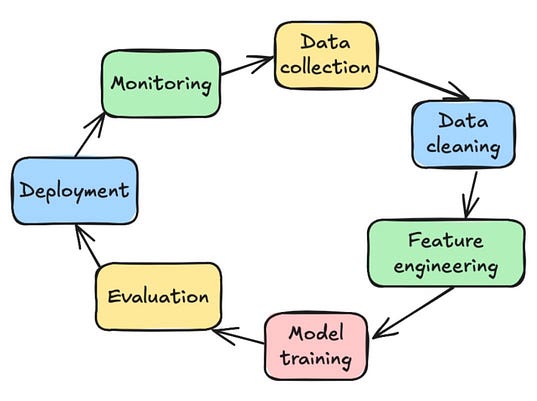
The machine learning life cycle

If you’ve been in the data science space for any amount of time, you’ve most likely heard this buzz term.

The machine learning life cycle.

It sounds fancy, but this is what it really boils down to:

• Machine learning is an active and dynamic process — it doesn’t have a strict beginning or end
• Once a model is trained and deployed, it will most likely need to be retrained as time goes on, thus restarting the cycle.
• There are steps within the cycle, however, that need to be followed in their proper order and executed carefully

When you Google the ML life cycle, each source will probably give you a slightly different number of steps and their names.

However, you will notice that for the most part, the cycle contains: problem definition, data collection and preprocessing, feature engineering, model selection and training, model evaluation, deployment, and monitoring.

1. Define problem

What is the problem you’re trying to solve or the question you’re trying to answer? Do you need machine learning or could you use a simpler approach (eg statistics)?

For the purposes of this article, I will follow a standard example that I’ve showcased quite a few times before: Hourly energy use forecasting.

• Problem: A client wants to be able to forecast a day of hourly consumption in order to identify trends in terms of which hours of the day and days of the week that consumption seems to be highest. They will use this information to find ways to cut back on usage throughout days and times that tend to have higher loads.
• Goal: To forecast the next 24 hours of electric energy consumption
• Methodology needed: Machine learning is needed for this task to increase accuracy. A simple model such as a moving average model would not take into account important features such as hour of day and day of week and wouldn’t be able to showcase the relationships between these features and the target variable.
• Data needed: Hourly consumption data with appropriate timestamps
• Amount of data needed: At least 1 year of historical data (The dataset we will be examining has 10 years of historical data, which is great)
• Explainability: We will need a model that is at least able to explain which features are contributing the most to the forecast
• Metrics: We want to achieve a MAPE (Mean Average Percent Error) of 10% or less on our test set. We also want to look at metrics such as RMSE and use this for model optimization and tuning.

2. Data collection

The dataset I will be using comes from Kaggle (CC0 public domain license). It is an hourly energy consumption dataset comprised of electric data. It contains a date/timestamp as well as the electric consumption in megawatts (MW).

In Python, the first thing you need to do is load your data into a DataFrame. I downloaded the dataset as a CSV from Kaggle and loaded it into my Python notebook script:

import pandas as pd

df = pd.read_csv("AEP_hourly.csv")

Calling df.head() will show you the first 5 rows of the DataFrame. It’s good to call this to check the overall structure of your data and see the columns you have.

The next step is to perform EDA (Exploratory Data Analysis). EDA involves:

• Exploring the data numerically via descriptive statistics & value counts
• Exploring the data visually via graphs and charts
• Making general initial inferences based on exploration

Here are some simple one-liners that you can use to kickstart the EDA process:

# Tells you the name and number of columns, the total number of rows,
# column data types, and the number of non-null/null values in the df
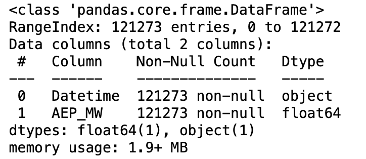
df.info()

Here’s the output for this dataset:

# Provides you with a dataframe containing descriptive statistics 
# such as the mean, standard deviation, and min/max values.
df.describe()

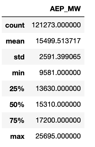
Another helpful one is df.value_counts(). This counts the number of unique values in your columns and tells you how many of each are present in the DataFrame (per column).

Since we aren’t dealing with categorical data, this isn’t as important for this dataset.

Visual EDA often involves inspecting the data visually in a variety of ways.

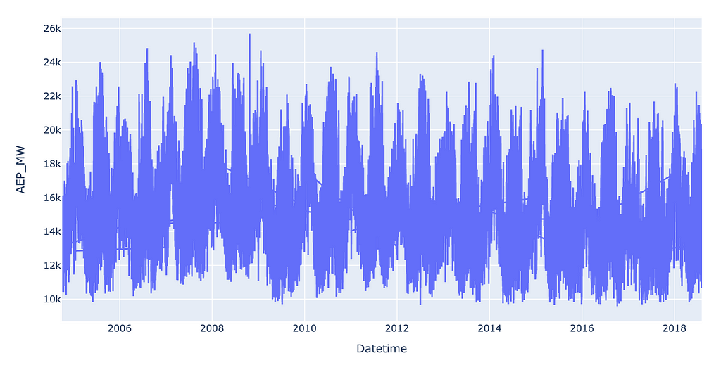
For a time series dataset like this one, one of the easiest places to start is simply plotting the data as a scatter or line chart.

import plotly.express as px

px.line(df, x=“Datetime”, y=“AEP_MW”)

Which produces this output:

Other common visualizations you can create for EDA purposes:

• Correlation plot between features and target
• Correlation plot between features and other features
• Linear regression scatter plot with regression line and R^2
• Trend and seasonality of time series data
• Autocorrelation plots for time series data

The type of EDA charts you produce have to do with the type of data you’re dealing with, so it really varies.

As a general rule, you want to look for trends in the data that could potentially affect which features you’ll include in your model later on.

3. Data cleaning and preprocessing

One thing I noticed right away is that the line chart I produced has random lines that reach across the screen, which means that some of the timestamps are out of order.

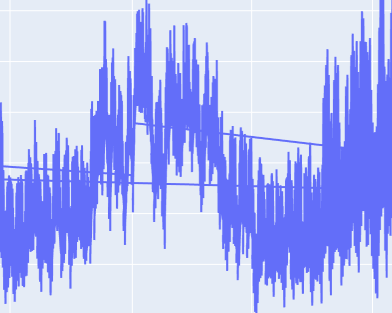
In order to resolve this, I cast the date time column to a pd.datetime object so I can call pandas specific functions on it. I then sort the column.

df[“Datetime”] = pd.to_datetime(df[“Datetime”])
# Set index to datetime so you can call sort_index function
df.set_index('Datetime',inplace=True)
df.sort_index(inplace=True)
# Reset the index so datetime is a regular column again
df.reset_index(inplace=True)

The graph now looks a lot better:

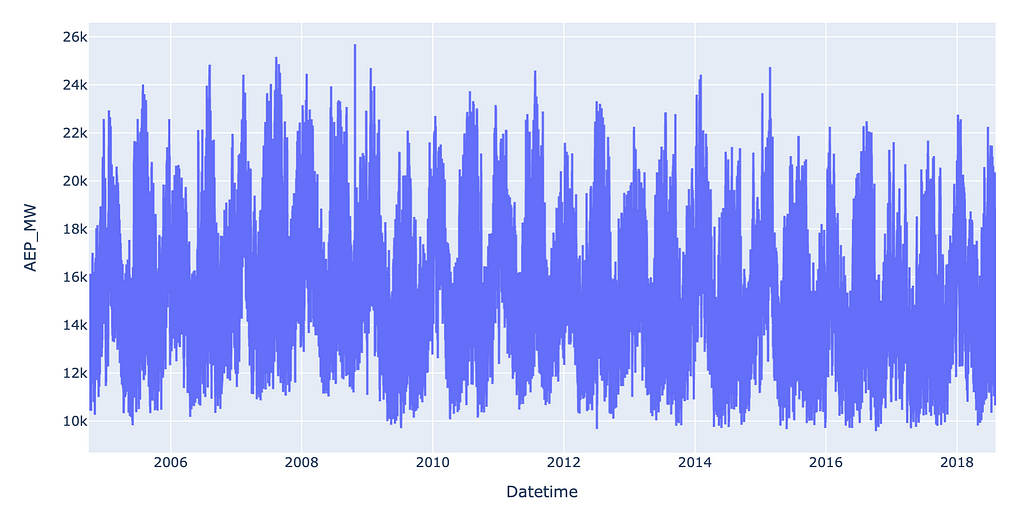
Another important thing to check for is missing or null values. In the case of time series data, you should also check for 0 values, and investigate whether or not they are valid entries or indicative of missing data.

Then, you can decide whether you need to remove missing values or impute them with the median or mean of the dataset.

For a more thorough exploration of the various ways to deal with missing data in a time series dataset, check out the following article:

How to: Handle Missing Data for Time Series

Handling outliers comes next.

Outliers must first be detected, and then either dropped or imputed, much like missing/null values.

A very simple way to identify outliers is z-score, which tells you how far away each data point is from the mean. If a data point has a z score > 3 or <-3 (meaning that the data point is 3 standard deviations above/below the mean), it is considered an outlier. You can tighten or loosen this threshold, however, based on your own judgment and analysis of the data.

from scipy import stats
# Create a separate z-score column 
df["z_score"]=stats.zscore(df["AEP_MW"])

# Once you have this z-score column, you can filter out 
# columns with a z-score > 3 or <-3
df = df[(df["z_score"]>3) | (df["z_score"]<-3)]]

# Drop z_score column from df since it is not a valid feature
df.drop("z_score",axis=1,inplace=True)

I explore more statistical methods for outlier detection in this article:

3 Simple Statistical Methods for Outlier Detection

4. Feature engineering

The next step is to select your features, prepare and optimize them for model consumption, split them into a train/test split framework and scale them as necessary.

Feature engineering is essentially the process of choosing and manipulating features in hopes of extracting as much relevant information from them to feed into a model.

Feature selection can be done manually or algorithmically. For the purposes of this problem, since the original DataFrame only comes with 1 feature column (the timestamp column), the amount of features we can create from this timestamp is limited.

We can’t feed a timestamp into a machine learning model because it doesn’t know how to read/process that information. Thus, we need to extract the time series features (such as hour, day, week) and encode them as numerical so the model can understand them.

Given an hourly timestamp column, we could extract:

• Hour of day
• Hour of week
• Hour of year
• Day of week
• Day of month
• Day of year
• Week of month
• Week of year
• Month of year
• Year

Of course, some of these features will overlap with each other. We don’t need both hour of week AND hour of day AND day of week. Hour of day and day of week OR just hour of week will probably be sufficient, and you can try out both combinations to see which yields the best performance.

We can extract these features as booleans (using a method such as one-hot encoding) or we can also encode them as cyclical time series features using sine and cosine:

Cyclical Encoding: An Alternative to One-Hot Encoding for Time Series Features

When it comes to time series features like “day of week”, transforming a datetime column into numerical values such as 1,2,3,…7 will also not work well with a time series ML model because technically these are categorical features, not numerical ones, even if we choose to represent them with numbers.

So we need to use a method called one-hot encoding, which essentially transforms categorical values as booleans using multiple columns as indicators.

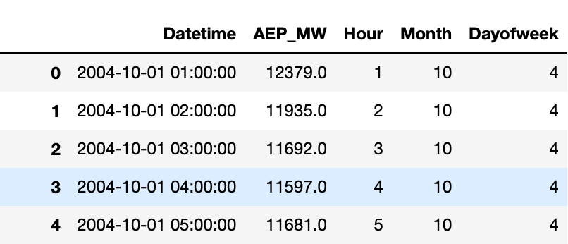
For the purposes of this article and to keep things simple, I’ll show you how I would transform the timestamp column into one-hot encoded time series features:

# I selected hour, month, and day of week to start.
# The code below transforms the datetime column into numerical columns.
# The same process applies to other features, depending on if the 
# .dt. has that feature (eg dt.year is a thing, but dt.hourofmonth is not)
# If you want hourofmonth, you'll have to calculate it yourself
df['Hour']=df['Datetime'].dt.hour
df['Month']=df['Datetime'].dt.month
df['Dayofweek']=df['Datetime'].dt.dayofweek

# Use pd.get_dummies to transform numerical columns into dummy variables
# (boolean values for each category)
columns_to_encode = ['Hour', 'Month', 'Dayofweek']
df = pd.get_dummies(df, columns=columns_to_encode,dtype=int)

Some models require you to scale any numerical features you have. Examples of these models include linear regressions, logistic regression, and neural networks.

Since we’re only using categorical features in our model, we won’t need to scale or standardize our features. If we had an additional feature, such as Temperature, which is numerical, depending on the type of model we select, we may need to scale that column.

Before you scale your features, it’s important that you first split your data into respective train/test sets. To do this, you could either use scikit-learn’s train_test_split method, which by default splits your data into 75% training and 25% testing — or, you can manually split the data up yourself.

An important thing to note is that scikit-learn’s train/test split randomly divides the dataset so that the rows are no longer in order.

This is not good practice for time series, so I’ve chosen to instead split the dataset up myself using indexing:

# Make the train set size 75% of the number of rows in the dataframe 
train_size = int(df.shape[0] * 0.75)

# Define features 
features = df.drop(["AEP_MW","Datetime"],axis=1).columns

# Split dataframe by train/test sets indices
df_train = df.iloc[0:train_size]
df_test = df.iloc[train_size:]

# Split dfs into separate arrays for features (X) and target (y)
X_train = df_train[features]
y_train = df_train["AEP_MW"]
X_test = df_test[features]
y_test = df_test["AEP_MW"]

For a deeper dive on scaling, normalization and standardization of data, check out this article:

Data Scaling 101: Standardization and Min-Max Scaling Explained

5. Model selection and training

It’s always good practice to train a baseline model before you train a final, more complex model. A baseline model would typically be a simpler version of the target model (for example, if you aim to train a Random Forest model, your baseline model can be a Decision Tree).

A baseline model helps to establish baseline metrics, such as a base MAPE, RMSE, MSE, etc.

You can compare these metrics against your more advanced model when the time comes which can help identify issues with the data, features, or hyperparameters.

Baseline Models in Time Series

Now you need to choose the best final model for your problem.

This will vary widely by field, dataset, computing resources, and goals.

For this example, I’ll choose a Random Forest model since it is one of the more well known ensemble models and tends to perform relatively well with time series data.

from sklearn.ensemble import RandomForestRegressor

rf = RandomForestRegressor() 
rf.fit(X_train,y_train)

6. Model evaluation and tuning

Once you’ve trained your model, you need to evaluate how good it is.

There are 2 main ways to evaluate your model: via cross validation and a test set.

The test set was already separated from the training data, so we will use our trained model to predict the test set.

However, the test set only contains the last 25% of data. We also want to get an idea of how the model will perform across a range of data with different weeks, months, hours, and even years.

This is where cross validation comes in.

Cross validation uses the entire train set and fits multiple models on smaller portions of the dataset, with smaller “test” sets in each round.

These test sets are technically referred to as evaluation sets.

Cross-validation usually performs 5 evaluations across a split training set and then averages the accuracy scores (RMSE, MSE, R2, MAPE or another metric(s) of your choosing) to give you a cross validation score.

Here’s an article which walks you through how to do cross validation with time series data:

How-To: Cross Validation with Time Series Data

The next step is to use your original model — the one trained on the entire dataset — to predict a hold out test set which the model has never seen or predicted on before.

This gives you the best picture as to how your model will perform on future, unseen data.

from sklearn.metrics import mean_squared_error
from sklearn.metrics import mean_absolute_percentage_error

# Call .predict on test set, passing in features only X_test
predicted_test = rf.predict(X_test)

# Calculate the RMSE
rmse = mean_squared_error(y_test.values,predicted_test,squared=False)

print(rmse)
# The RMSE for our test set was 1799

# Calculate MAPE
mape = mean_absolute_percentage_error(y_test, predicted_test)
# Format MAPE into a percentage and print
print(f"MAPE: {mape * 100:.2f}%")
# Our initial MAPE was 10.36%, which is within range of 
# what we were hoping for!

Once you have calculated metrics for your cross validation and test set, it’s time for model tuning and optimization.

First, you want to ensure that you are not overfitting or underfitting.

In simple terms:

Overfitting is when your train set/cross validation accuracy is much better than your test set accuracy.

Underfitting is the opposite. If your model is underfitting, the accuracy on your training set will be poor. This basically means that the model didn’t properly learn patterns from the training set.

There are a few ways to deal with over and underfitting. One of the most well known ways is hyperparameter tuning, which is also just a standard technique to use even if your model performed well off the bat.

In our example, the cross-validation score for our train set was 1549. The test set score was 1799. These numbers are large because we are dealing with large values in the dataset in general (Mean: 15,499). There’s not a huge discrepancy between the test and CV scores, so I’m not too concerned about our model over or underfitting.

Hyperparameter tuning is the final tweaking step for optimizing your model’s performance and getting your metrics to the best possible values.

Here’s an example of one of the simplest hyperparameter tuning techniques, called grid search:

from sklearn.model_selection import GridSearchCV

# Define hyperparameters to tune
param_grid = {
    'n_estimators': [100, 200, 300],  
    'max_depth': [None, 10, 20, 30],  
    'min_samples_split': [2, 5, 10] 
}

# Define grid search cv object
grid_search = GridSearchCV(estimator=rf, param_grid=param_grid, 
                           cv=5, n_jobs=-1, verbose=2, 
                           scoring='neg_root_mean_squared_error')

# Fit the grid search object - this will likely take a long time
# if the dataset is large and if you have defined lots of hyperparameters
grid_search.fit(X_train, y_train)

# Print the best hyperparameters found by GridSearchCV
print("Best Hyperparameters: ", grid_search.best_params_)

Grid search is known for being simple, yet slow. Random search is a faster option. Bayesian optimization is another faster and more intelligent option.

Once you have gotten the optimal hyperparameters according to grid search, random search or Bayesian search, you should get new test set metrics to ensure they have really improved your models.

# Evaluate the best model on the test set
# Get the best model from grid search object
best_rf = grid_search.best_estimator_
# Predict test set metrics using the best model
y_pred = best_rf.predict(X_test)

# Get the RMSE for the best model
rmse_best_rf = mean_squared_error(y_test.values,y_pred,squared=False)

print(rmse_best_rf)

Bayesian Optimization: Faster hyperparameter tuning in Python

Model evaluation may also include examining model explainability — in the case of Random Forest, looking at feature importances.

Feature importances tell you which features are contributing the most to the model’s predictions.

# Getting feature importances for each feature for Random Forest model
feature_names = X_train.columns
feature_importances = rf.feature_importances_

# Create feature importance df with names and importance values
df_importance = pd.DataFrame({
    'Feature': feature_names,
    'Importance': feature_importances
})

# Sort the DataFrame by importance (descending order)
df_importance = df_importance.sort_values(by='Importance', ascending=False)

7. Model deployment

Amazing — you made it through data collection, cleaning, engineering, model training, evaluation and tuning, and you have a trained model that performs well according to the standards you set in the planning phase.

Now what happens?

Well, you need to make this model available to anyone and everyone who needs it, and not just available to you and your Jupyter notebook.

Model deployment is essentially the process of integrating a trained ML model into a production environment where it can make real-time predictions or otherwise support decision-making.

Deployment involves:

• Saving the model in a deployable format (e.g. pickle).
• Setting up an environment, such as a cloud platform (e.g., AWS, GCP) and/or containerization tool (e.g., Docker), to host the model.
• Exposing the model to users via a web server or application.

Model deployment is a complicated process and it definitely has a learning curve. It’s too much for me to cover in this article specifically, though I may cover it sometime in the near future in an upcoming article.

For more detailed information on model deployment, check out this informative article.

8. Model monitoring

So you’ve deployed your model.

But the job is far from over.

As new data comes in, circumstances change and metrics are updated, you’ll have to be ready to update your model as necessary.

Model monitoring involves tracking the performance and behavior of a machine learning model to ensure it continues to perform as expected in a production environment.

Over time, models can start to decay — meaning that as data patterns change, the original model is no longer able to predict as well as it did before.

Metrics like mean absolute error (MAE) or mean squared error (MSE) can be calculated regularly to detect decay.

A dashboard is a great way to monitor data patterns over time as well as track metrics and flag anomalies.

Alerts can be set up to flag unusual behavior (such as consistent over- or under-predictions) and then trigger automatic or manual model retraining.

I discuss model decay and retraining more in depth here:

What is Model Decay?

Conclusion

Notice how the final step, monitoring, will often end in model retraining. This starts you back at square 1.

Defining new problem and goals, collecting new data (or the same data but perhaps with the intention to engineer it differently), and ultimately retraining and redeploying the model.

So you can see how machine learning is not a one and done type of task — it truly is a cycle.

It’s also important to note that the cycle can restart at any point in the process, not just at the end.

For example, if your model was found to be overfitting during the evaluation phase, you might gather data again, engineer the features differently, and choose new hyperparameters, moving you back steps in the cycle or starting it over.

I will say that it takes a long time to truly memorize all these steps in their proper order and truly understand them.

And there’s a lot more nuance to each of the steps I listed above — it varies greatly by the type of model, the problem you’re solving and more.

But the best way is to continue to practice and learn through repetition.

Thanks for reading

Find the source code and dataset here | Connect with me on LinkedIn!

Get an email whenever Haden Pelletier publishes.

---

Every Step of the Machine Learning Life Cycle Simply Explained was originally published in Towards Data Science on Medium, where people are continuing the conversation by highlighting and responding to this story.

from Datascience in Towards Data Science on Medium https://ift.tt/IPgTQbs
via IFTTT