Histogram of Oriented Gradients (HOG) in Computer Vision
An explanation and implementation of Histogram of Oriented Gradients (HOG) (feature extraction algorithm ) for object detection and recognition tasks
Introduction
Histogram of Oriented Gradients was first introduced by Navneet Dalal and Bill Trigs in their CVPR paper [“Histograms of Oriented Gradients for Human Detection”]
There are many different algorithms for feature extraction, depending on the type of features it focuses on, such as texture, color, or shape, whether it describes the image as a whole or just local information.
The HOG algorithm is one of the most essential techniques in feature extraction as it is a fundamental step for object detection and recognition tasks.
In this article, we will explore the principles and implementation of the HOG algorithm.
What is a Histogram of Oriented Gradients (HOG)?
The HOG is a global descriptor (feature extraction) method applied to each pixel within an image to extract neighborhood information(neighborhood of pixel) like texture and compress/abstract that information from a given image into a reduced/condensed vector form called a feature vector that could describe the feature of this image which is very useful when it came to captures edge and gradient structures in an image. Moreover, we can compare this processed image for object recognition or object detection.
The HOG Explanation
1- Calculate the Gradient Image
To extract and capture edge information, we apply a Sobel operator consisting of two small matrices (filter/kernel) that measure the difference in intensity at grayscale(wherever there is a sharp change in intensity).
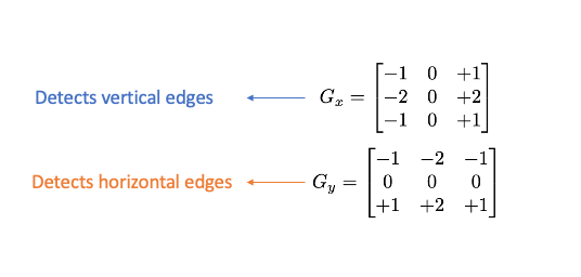
We apply this kernel on pixels of the image by convolution :
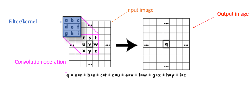
After applying Sobel Kernel to the image now, we can calculate the magnitude and orientation of an image :

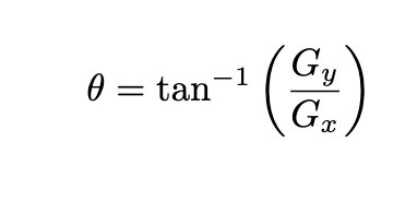
The gradients determine the edges' strength (magnitude) and direction (orientation) at a specific point. The edge direction is perpendicular to the gradient vector’s direction at the location where the gradient is calculated. In other words, the length and direction of the vector.
2- Calculate the Histogram of the Gradient
For each pixel, we have two values: magnitude and orientation. To combine this information into something meaningful, we use a histogram, which helps organize and interpret these values effectively.
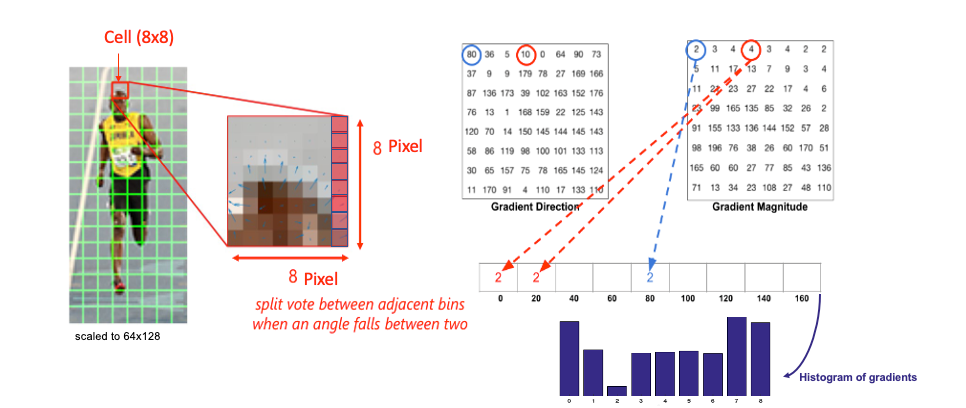
We create a histogram of gradients in these cells ( 8 x 8 ), which have 64 values distributed to bins in the histogram, which are quantized into 9 bins each of 20 degrees ( spanning 0° to 180°). Each pixel's magnitude value (edge strength) is added as a “vote” to the corresponding orientation bin so the histogram's peaks reveal the pixel's dominant orientations.
3- Normalization
Since gradient magnitudes depend on lighting conditions, normalization scales the histograms to reduce the influence of lighting and contrast variations.
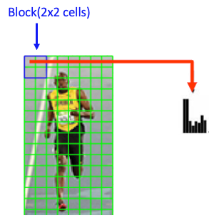
Each block typically consists of a grid of cells (2x2). This block slides across the image with overlap, meaning each cell is included in multiple blocks.
Each block has 4 histograms ( 4 cells ), which can be concatenated to form a 4(cells) x 9 (bins )x1 vector = 36 x 1 element vector for each block; overall image in the example: 7 rows x 15 cols = 7x15x36=3780 elements. This feature vector is called the HOG descriptor, and the resulting vector is used as input for classification algorithms like SVM.
# we will be using the hog descriptor from skimage since it has visualization tools available for this example
import cv2
import matplotlib.pyplot as plt
from skimage import color, feature, exposure

# Load the image
img = cv2.imread('The path of the image ..')

# Convert the original image to RGB
img_rgb = cv2.cvtColor(img, cv2.COLOR_BGR2RGB)

# Convert the original image to gray scale
img_gray = cv2.cvtColor(img_rgb,cv2.COLOR_RGB2GRAY)

plt.imshow(img_gray,cmap="gray")

# These are the usual main parameters to tune in the HOG algorithm.
(H,Himage) = feature.hog(img_gray, orientations=9, pixels_per_cell=(8,8), cells_per_block=(2,2),visualize=True)

Himage = exposure.rescale_intensity(Himage, out_range=(0,255))
Himage = Himage.astype("uint8")

fig = plt.figure(figsize=(15, 12), dpi=80)
plt.imshow(Himage)
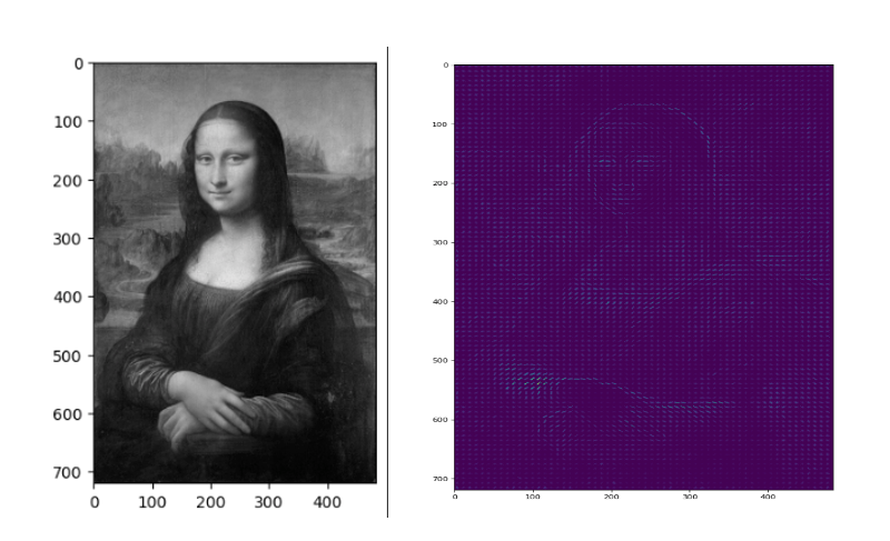
As you can see, HOG effectively captures the general face shape (eyes, nose, head) and hands. This is due to HOG’s focus on gradient information across the image, making it highly effective for detecting lines and shapes. Additionally, we can observe the dominant gradients and their intensity at each point in the image.
(HOG) algorithm for human detection in an image
HOG is a popular feature descriptor in computer vision, particularly effective for detecting shapes and outlines, such as the human form. This code leverages OpenCV’s built-in HOG descriptor and a pre-trained Support Vector Machine (SVM) model specifically trained to detect people
# Load the image
img = cv2.imread('The path of the image ..')

# Convert the original image to RGB
img_rgb = cv2.cvtColor(img, cv2.COLOR_BGR2RGB)

# Convert the original image to gray scale
img_gray = cv2.cvtColor(img_rgb,cv2.COLOR_RGB2GRAY)

#Initialize the HOG descriptor and set the default SVM detector for people
hog = cv2.HOGDescriptor()
hog.setSVMDetector(cv2.HOGDescriptor_getDefaultPeopleDetector())

# Detect people in the image using the HOG descriptor
bbox, weights = hog.detectMultiScale(img_gray ,winStride = (2,2), padding=(10,10),scale=1.02)

# Draw bounding boxes around detected people
for (x, y, w, h) in bbox:
    cv2.rectangle(img_rgb, (x, y),
                  (x + w, y + h),
                  (255, 0, 0), 4)

plt.imshow(img_rgb)
After loading the test image, we use HOG’s detectMultiScale method to detect people, with winStride set to skip one pixel per step, improving speed by trading off a bit of accuracy, which is crucial in object detection since it is a computationally intensive process. Although the detector may identify all people, sometimes there’s a false positive where part of one person’s body is detected as another person. To fix this, we can apply Non-Maxima Suppression (NMS) to eliminate overlapping bounding boxes, though bad configuration(winterize, padding, scale) can occasionally fail to detect objects.
Wrap-up
wrap --up The HOG descriptor computation involves several steps:
1. Gradient Computation
2. Orientation Binning
3. Descriptor Blocks
4. Normalization
5. Feature Vector Formation
In this article, we explored the math behind HOG and how easy it is to apply in just a few lines of code, thanks to OpenCV! I hope you found this guide helpful and enjoyed working through the concepts. Thanks for reading, and see you in the next post!
References
- L. Daudet, B. Izrar, and R. Motreff, Histograms of Oriented Gradients for Human Detection(2010), HAL open science.
- Satya Mallick, Image Recognition and Object Detection: Part 1,2016, learn OpenCV.
- Satya Mallick, Histogram of Oriented Gradients explained using OpenCV , 2016, learn OpenCV
Histogram of Oriented Gradients (HOG) in Computer Vision was originally published in Towards Data Science on Medium, where people are continuing the conversation by highlighting and responding to this story.
from Datascience in Towards Data Science on Medium https://ift.tt/F0GBkIA
via IFTTT


