Increase Trust in Your Regression Model The Easy Way
How to use Conformalized Quantile Regression

We must know how sure our model is about its predictions to make well-informed decisions. Hence, returning only a point prediction is not enough. It does not tell us anything about whether we can trust our model or not. If you want to know why, check out my article below.
Uncertainty Quantification and Why You Should Care
In the article, I use a classification problem as an example. However, many real-world problems are regression problems. For example, we want to know how certain a model is when predicting tomorrow’s temperature.
As the temperature is a continuous variable, we would like to know in which interval the true temperature will lie.
The wider the interval, the more uncertain the model. Hence, we should trust it less when making decisions.
But how do we get such a prediction interval?
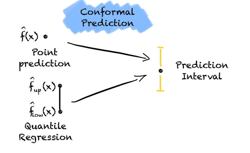
Two approaches come to mind. Either we use a set of models that predict the interval or we turn a point prediction into a prediction interval.
Let’s start with the first approach also known as quantile regression.
We fit two models on the data, one low-quantile regressor and one high-quantile regressor. Each regressor estimates a conditional quantile of the target variable. Combining these two gives us our prediction interval.
The main advantage is that we can use any model architecture for quantile regression by using the Pinball loss function. But, the main disadvantage is that the prediction interval is not calibrated. There is no guarantee that the true value will lie in the interval with a predefined probability. As the interval is thus not reliable, we should not put too much trust into the interval. Particularly, for critical downstream decisions.
Let’s see if the second approach is better.
In previous articles, I described how Conformal Prediction turns point predictions into prediction sets and guarantees coverage for classification problems.
Luckily Conformal Prediction doesn’t stop there. Conformal Prediction is a framework that can be wrapped around any prediction model. Hence, we can apply Conformal Prediction and the same steps as we do for classification problems. The only difference is the non-conformity score. Hence, if you have read my other articles you should be familiar with the process.

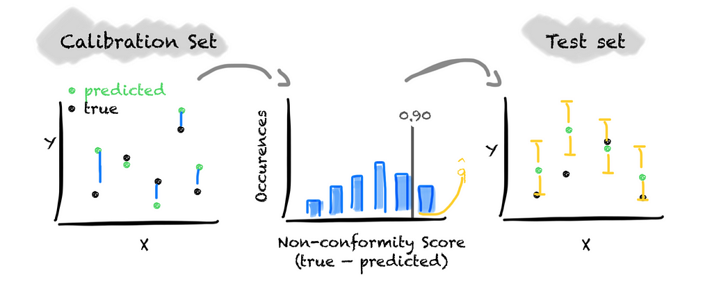
First, we choose a significance level alpha and a non-conformity score. As the non-conformity score, we use the forecast error, i.e., y_true — y_pred. Second, we split the dataset into a train, calibrate, and test subset. Third, we train the model on the training subset of the dataset. Fourth, we calibrate the model on the calibration subset of the data. For this, we calculate the non-conformity score, i.e., the prediction error. Based on the distribution of the non-conformity score, we determine the threshold that covers 1-alpha values. To form the prediction interval for unseen data, we add and subtract the threshold from the predicted value.
That’s it. We have turned a point prediction into a calibrated prediction interval.
Although the approach is straightforward, it has one big disadvantage. The prediction interval is not adaptive. The prediction interval has always the same width. It does not adapt to different regions of the feature space. Hence, it does not state which data points are harder to predict.
So, what now?
We have two approaches. One is adaptive but not calibrated (quantile regression). The other is not adaptive but calibrated (conformal prediction). Can we combine them to receive adaptive prediction intervals with guaranteed coverage?
This is exactly what Conformalized Quantile Regression does. The approach was first published in 2019.
How does Conformalized Quantile Regression work?
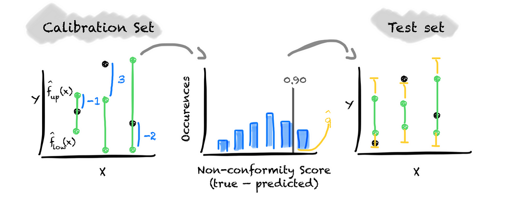
It is quite easy. We wrap Conformal Prediction around a quantile regression, adjusting the interval. With this, we calibrate (or conformalize) the prediction interval of the quantile regression. To calibrate the quantile regression model, we determine a factor by which we extend or shrink the interval.
For this, we apply the same steps as earlier. Again, the only difference is the non-conformity score we choose. We now deal with an interval instead of a point prediction. Hence, we define the non-conformity score as the difference between the true value and its nearest predicted quantile, i.e., max(lb-y, y-ub).
If the true value lies between the predicted quantiles, the non-conformity score is negative. If the true values fall outside the predicted interval, the non-conformity score is positive.

We then build the distribution of the non-conformity score and determine the threshold that covers 1 — alpha values. If the threshold value is positive we need to grow the predicted interval while we shrink it if the value is negative. We do this by adding the value to the upper quantile and subtracting it from the lower quantile.
That’s how easy it is. We now have an adaptive prediction interval that guarantees coverage for regression problems.
Conclusion
In this article, I have shown you an approach to quantifying the uncertainty in regression problems.
If you stayed until here, you now should…
- have an understanding of how to use Conformal Prediction for regression problemns and
- be able to use Conformalized Qunatile Regression in practice.
If you want to dive deeper into Conformalized Quantile Regression, check out the paper. Otherwise, comment and/or see you in my next article.
Obviously there are many more Conformal Prediction approaches for regression tasks and timeseries forecasting in particular, such as EnbPI, or Adaptive Conformal Inference (ACI). So, stay tuned for my next articles.
Increase Trust in Your Regression Model The Easy Way was originally published in Towards Data Science on Medium, where people are continuing the conversation by highlighting and responding to this story.
from Datascience in Towards Data Science on Medium https://ift.tt/T5lSwCi
via IFTTT

