NLP Illustrated, Part 2: Word Embeddings
An illustrated and intuitive guide to word embeddings
Welcome to Part 2 of our NLP series. If you caught Part 1, you’ll remember that the challenge we’re tackling is translating text into numbers so that we can feed it into our machine learning models or neural networks.
NLP Illustrated, Part 1: Text Encoding
Previously, we explored some basic (and pretty naive) approaches to this, like Bag of Words and TF-IDF. While these methods get the job done, we also saw their limitations — mainly that they don’t capture the deeper meaning of words or the relationships between them.
This is where word embeddings come in. They offer a smarter way to represent text as numbers, capturing not just the words themselves but also their meaning and context.
Let’s break it down with a simple analogy that’ll make this concept super intuitive.
Imagine we want to represent movies as numbers. Take the movie Knives Out as an example.
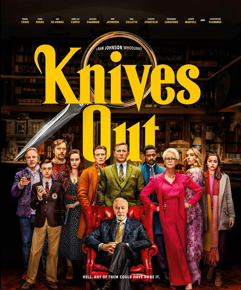
We can represent a movie numerically by scoring it across different features, such as genres — Mystery, Action, and Romance. Each genre gets a score between -1 and 1 where: -1 means the movie doesn’t fit the genre at all, 0 means it somewhat fits, and 1 means it’s a perfect match.
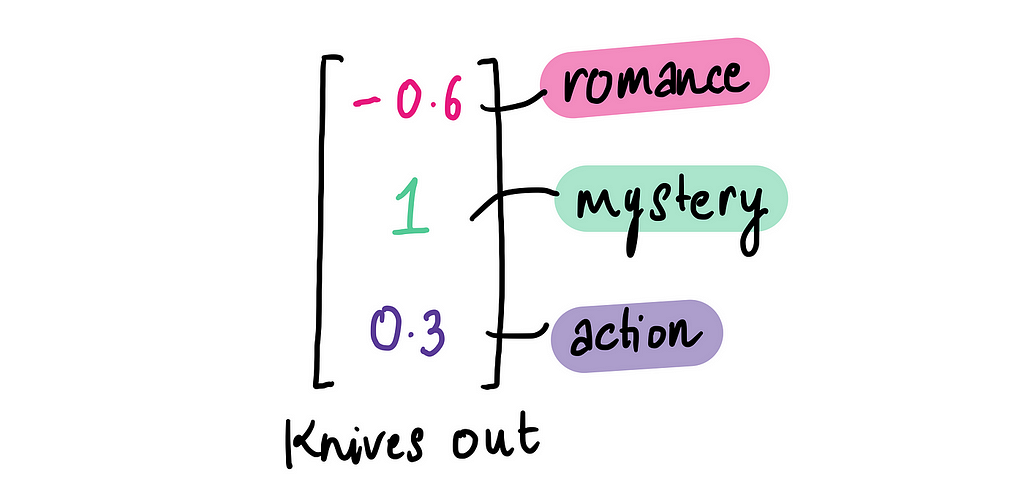
So let’s start scoring Knives Out! For Romance, it scores -0.6 — there’s a faint hint of romance, but it’s subtle and not a big part of the movie, so it gets a low score.

Moving on to Mystery, it’s a strong 1 since the entire movie revolves around solving a whodunit. And for Action, the movie scores 0.2. While there is a brief burst of action toward the climax, it’s minimal and not a focal point.
This gives us three numbers that attempt to encapsulate Knives Out based these features: Romance, Mystery, and Action.

Now let’s try visualizing this.
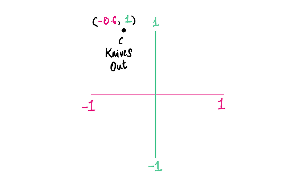
If we plot Knives Out on just the Romance scale, it would be a single point at -0.6 on the x-axis:

Now let’s add a second dimension for Mystery. We’ll plot it on a 2D plane, with Romance (-0.6) on the x-axis and Mystery (1.0) on the y-axis.
Finally, let’s add Action as a third dimension. It’s harder to visualize, but we can imagine a 3D space where the z-axis represents Action (0.3):
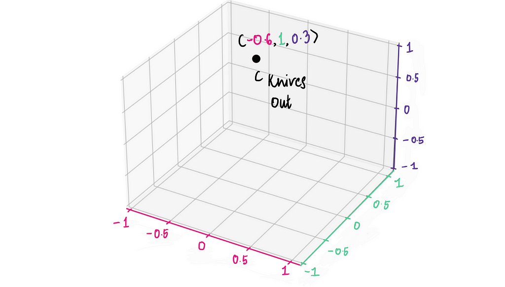
This vector (-0.6, 1, 0.3) is what we call a movie embedding of Knives Out.
Now let’s take another movie as an example: Love Actually.

Using the same three features — Romance, Mystery, and Action — we can create a movie embedding for it like so:
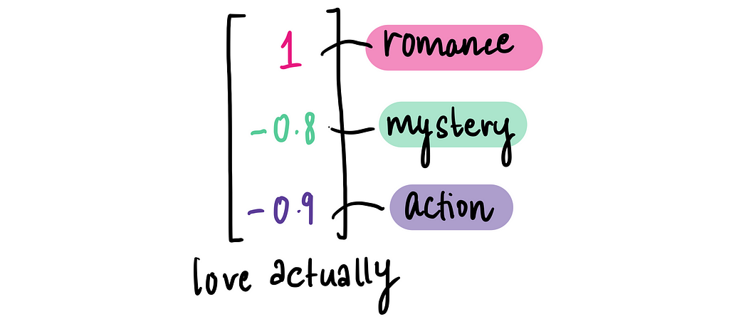
And we can plot this on our movie embeddings chart to see how Love Actually compares to Knives Out.
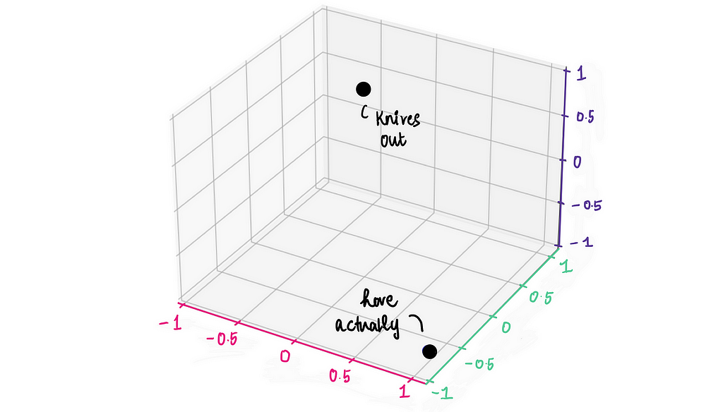
From the graph, it’s obvious that Knives Out and Love Actually are super different. But what if we want to back this observation with some numbers? Is there a way to math-ify this intuition?
Luckily, there is!
Enter cosine similarity. When working with vectors, a common way to measure how similar two vectors are is by using cosine similarity. Simply put, it calculates the similarity by measuring the cosine of the angle between two vectors. The formula looks like this:
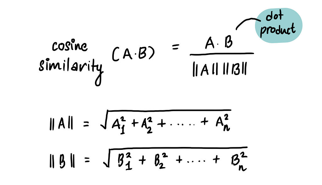
Here, A and B are the two vectors we’re comparing. A⋅B is the dot product of the two vectors, and ∥A∥ and ∥B∥ are their magnitudes (lengths).
Cosine similarity gives a result between -1 and 1, where:
- 1 means the vectors are identical (maximum similarity)
- -1 means they are completely opposite (no similarity)
From the graph, we’ve already observed that Knives Out and Love Actually seem very different. Now, let’s quantify that difference using cosine similarity. Here, vector A represents the embedding for Knives Out and vector B represents the embedding for Love Actually.

Plugging the values into the cosine similarity formula, we get:

And this result of -0.886 (very close to -1) confirms that Knives Out and Love Actually are highly dissimilar. Pretty cool!
Let’s test this further by comparing two movies that are extremely similar. The closest match to Knives Out is likely its sequel, The Glass Onion.
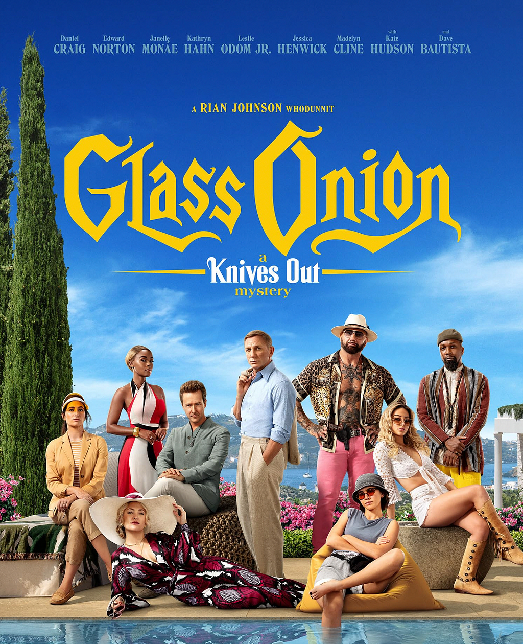
Here’s the movie embedding for The Glass Onion:
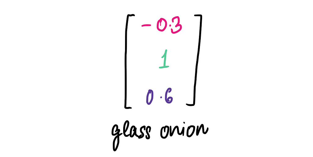
The embedding is slightly different from Knives Out. The Glass Onion scores a little higher in the Action category than in its predecessor, reflecting the increased action sequences of the sequel.
Now, let’s calculate the cosine similarity between the two movie embeddings:

And voilà — almost a perfect match! This tells us that Knives Out and The Glass Onion are extremely similar, just as we expected.
This movie embedding is a great start, but it’s far from perfect because we know movies are much more complex than just three features.
But we could make the embedding better by expanding the features. We can then capture significantly more nuance and detail about each film. For example, along with Romance, Mystery, and Action, we could include genres like Comedy, Thriller, Drama, and Horror, or even hybrids like RomCom.
Beyond genres, we could include additional data points like Rotten Tomatoes Score, IMDb Ratings, Director, Lead Actors, or metadata such as the film’s release year or popularity over time. The possibilities are endless, giving us the flexibility to design features as detailed and nuanced as needed to truly represent a movie’s essence.
Let’s switch gears and see how this concept applies to word embeddings. With movies, we at least had a sense of what our features could be — genres, ratings, directors, and so on. But when it comes to all words, the possibilities are so vast and abstract that it’s virtually impossible for us to define these features manually.
Instead, we rely on our trusted friends — the machines (more specifically neural networks) — to figure it out for us. We’ll dive deeper into how machines create these embeddings soon, but for now, let’s focus on understanding and visualizing the concept.
Each word can be represented as a set of numerical values (aka vectors) across several hidden features or dimensions. These features capture patterns such as semantic relationships, contextual usage, or other language characteristics learned by machines. These vectors are what we call word embeddings.
📣 This is important, so I’m going to reiterate: Word embeddings are vector representations of words.
For a very, very naive word embedding, we might start with just three features — similar to how we began with movies.

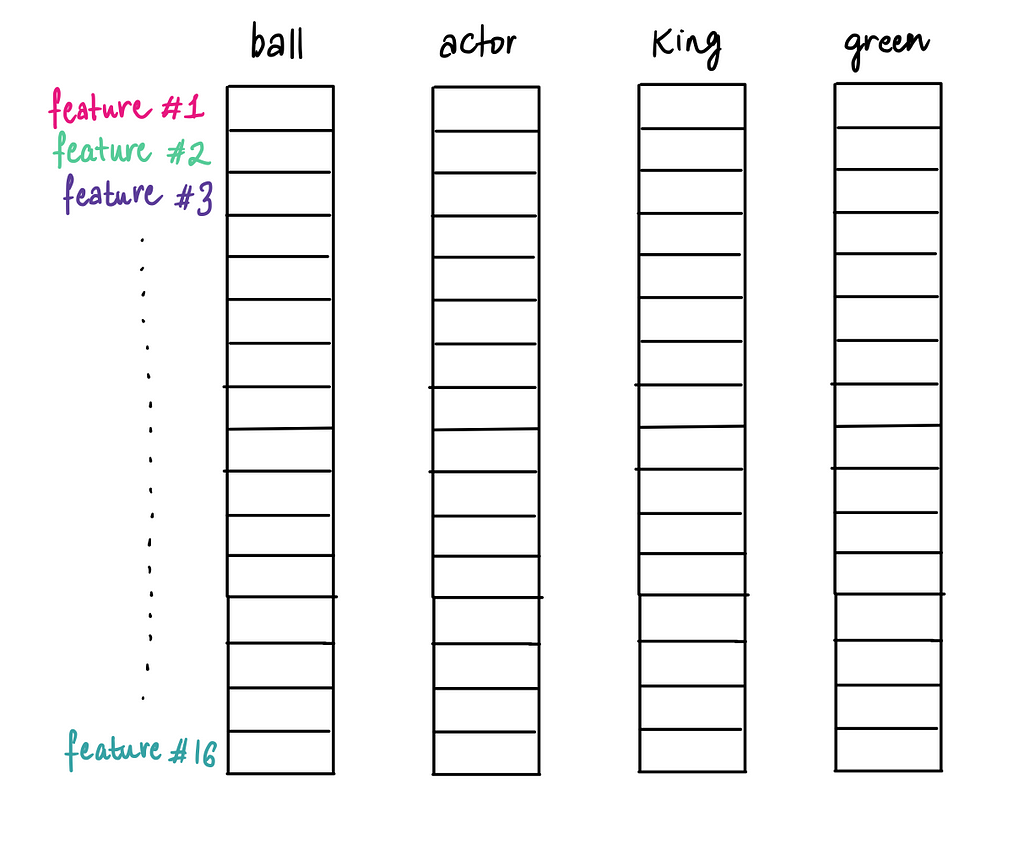
We can turn up the heat by expanding to 16 features, capturing more nuanced properties of words.
Or, we could take it even further with 200 features, creating a highly detailed and rich representation of each word.
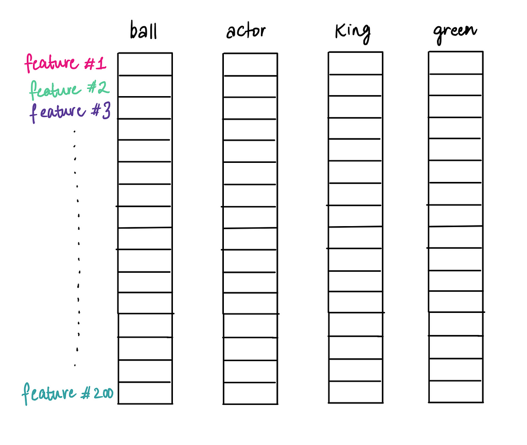
The more features we add, the more complex and precise the embedding becomes, enabling it to capture subtle patterns and meanings in language.
The idea behind word embeddings is simple yet powerful: to arrange words in such a way that those with similar meanings or usage are placed close to each other in the embedding space. For example, words like “king” and “queen” would naturally cluster together, while “apple” and “orange” might form another cluster, far away from unrelated words like “car” or “bus.”
While it’s impossible to visualize embeddings with 32 or more dimensions, conceptually, we can think of them as a high-dimensional space where words are grouped based on their relationships and meanings. Imagine it as a vast, invisible map where words with similar meanings are neighbors, capturing the intricate structure of language.
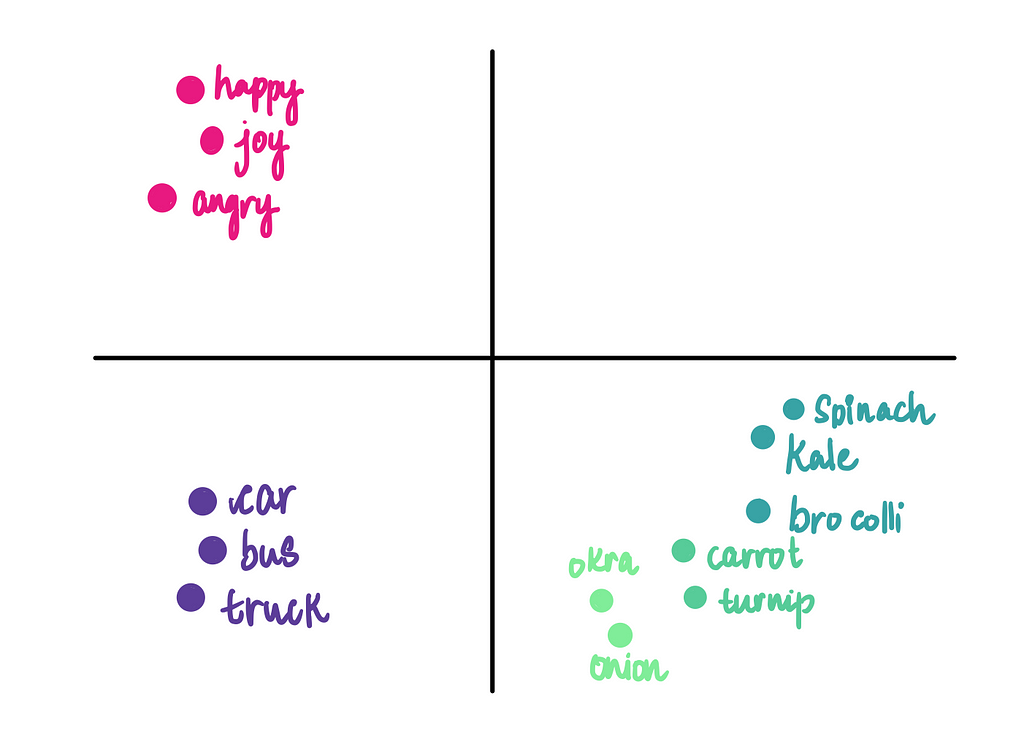
This clustering is what makes embeddings so effective in capturing the subtleties of language.
Another cool feature of word embeddings is that we can perform mathematical operations with them, leading to interesting and often intuitive results. One of the most famous examples is:

Just to illustrate this, let’s say we have the following 3-dimensional word embeddings for the words:
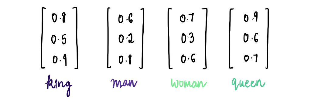
Using these embeddings, we can perform the operation: “king” — “man” + “woman”…

…which gives us the word embedding for “queen”!
Or we could have relationships like this:

…or even:

You get the idea. This works because word embeddings capture relationships between words in a mathematically consistent way. That’s what makes embeddings so powerful — they don’t just measure similarity; they encode meaningful relationships that mirror our human understanding of language.
Now, the big question is: how do we come up with word embeddings for each word? As mentioned earlier, the answer lies in leveraging the power of neural networks! These models learn the relationships and features of words by analyzing MASSIVE amounts of text data. And by doing so, we can see these patterns emerge naturally during the training process.
In the next article, we’ll see how neural networks do that by diving into one of the most popular word embedding models: Word2Vec!
In the meantime, if you’d like to dive deeper into Neural Networks, I have a series on Deep Learning that breaks down the math behind how they work.
Feel free to connect with me on LinkedIn or email me at shreya.statistics@gmail.com!
Unless specified, all images are by the author.
NLP Illustrated, Part 2: Word Embeddings was originally published in Towards Data Science on Medium, where people are continuing the conversation by highlighting and responding to this story.
from Datascience in Towards Data Science on Medium https://ift.tt/LfCihtV
via IFTTT


