Quantizing Neural Network Models
Understanding post-training quantization, quantization-aware training, and the straight through estimator

Large AI models are resource-intensive. This makes them expensive to use and very expensive to train. A current area of active research, therefore, is about reducing the size of these models while retaining their accuracy. Quantization has emerged as one of the most promising approaches to achieve this goal.
The previous article, Quantizing the Weights of AI Models, illustrated the arithmetics of quantization with numerical examples. It also discussed different types and levels of quantization. This article discusses the next logical step — how to get a quantized model starting from a standard model.
Broadly, there are two approaches to quantizing models:
- Train the model with higher-precision weights and quantize the weights of the trained model. This is post-training quantization (PTQ).
- Start with a quantized model and train it while taking the quantization into account. This is called Quantization Aware Training (QAT).
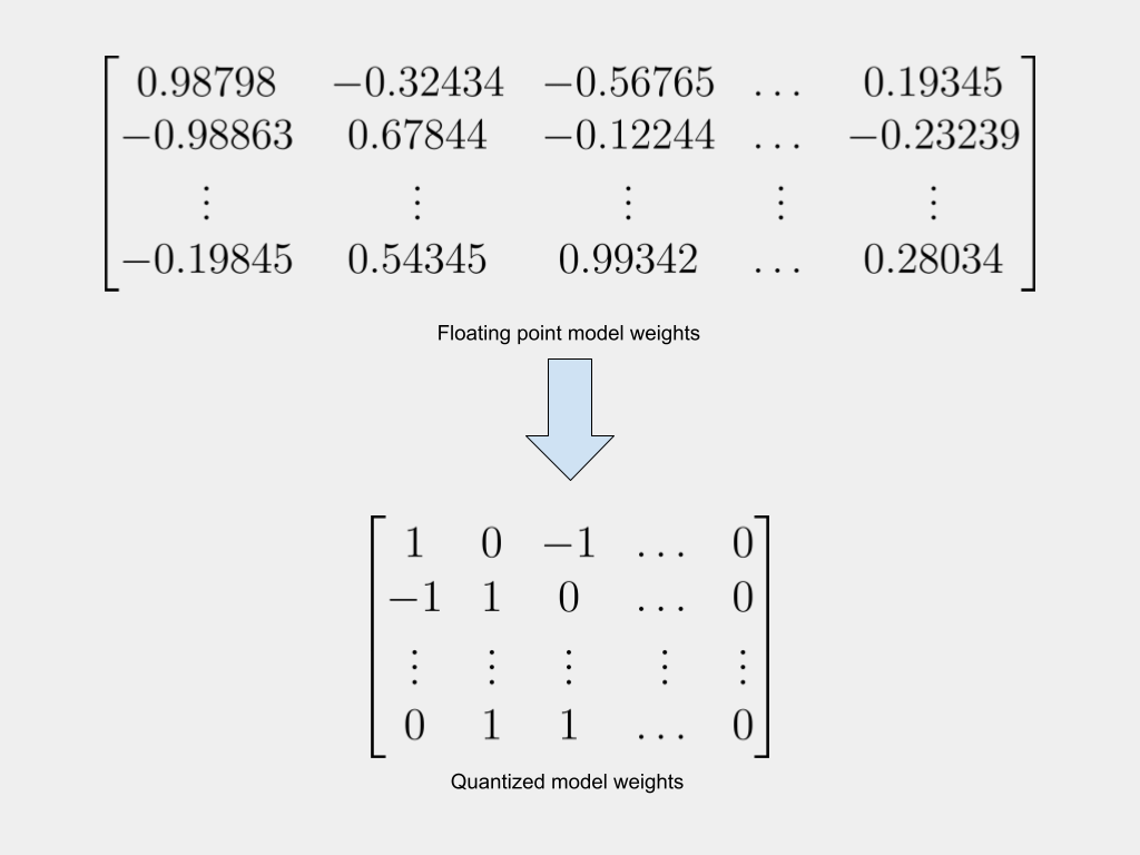
Since quantization involves replacing high-precision 32-bit floating point weights with 8-bit, 4-bit, or even binary weights, it inevitably results in a loss of model accuracy. The challenge, therefore, is how to quantize models, while minimizing the drop in accuracy.
Because it is an evolving field, researchers and developers often adopt new and innovative approaches. In this article, we discuss two broad techniques:
- Quantizing a Trained Model — Post-Training Quantization (PTQ)
- Training a Quantized Model — Quantization Aware Training (QAT)
Quantizing a Trained Model — Post-Training Quantization (PTQ)
Conventionally, AI models have been trained using 32-bit floating point weights. There is already a large library of pre-trained models. These trained models can be quantized to lower precision. After quantizing the trained model, one can choose to further fine-tune it using additional data, calibrate the model’s parameters using a small dataset, or just use the quantized model as-is. This is called Post-Training Quantization (PTQ).
There are two broad categories of PTQ:
- Quantizing only the weights
- Quantizing both weights and activations.
Weights-only quantization
In this approach, the activations remain in high precision. Only the weights of the trained model are quantized. Weights can be quantized at different granularity levels (per layer, per tensor, etc.). The article Different Approaches to Quantization explains granularity levels.
After quantizing the weights, it is also common to have additional steps like cross-layer equalization. In neural networks, often the weights of different layers and channels can have very different ranges (W_max and W_min). This can cause a loss of information when these weights are quantized using the same quantization parameters. To counter this, it is helpful to modify the weights such that different layers have similar weight ranges. The modification is done in such a way that the output of the activation layers (which the weights feed into) is not affected. This technique is called Cross Layer Equalization. It exploits the scale-equivariance property of the activation function. Nagel et al., in their paper Data-Free Quantization Through Weight Equalization and Bias Correction, discuss cross-layer equalization (Section 4) in detail.
Weights and Activation quantization
In addition to quantizing the weights as before, for higher accuracy, some methods also quantize the activations. Activations are less sensitive to quantization than weights are. It is empirically observed that activations can be quantized down to 8 bits while retaining almost the same accuracy as 32 bits. However, when the activations are quantized, it is necessary to use additional training data to calibrate the quantization range of the activations.
Advantages and disadvantages of PTQ
The advantage is that the training process remains the same and the model doesn’t need to be re-trained. It is thus faster to have a quantized model. There are also many trained 32-bit models to choose from. You start with a trained model and quantize the weights (of the trained model) to any precision — such as 16-bit, 8-bit, or even 1-bit.
The disadvantage is loss of accuracy. The training process optimized the model’s performance based on high-precision weights. So when the weights are quantized to a lower precision, the model is no longer optimized for the new set of quantized weights. Thus, its inference performance takes a hit. Despite the application of various quantization and optimization techniques, the quantized model doesn’t perform as well as the high-precision model. It is also often observed that the PTQ model shows acceptable performance on the training dataset but fails to on new previously unseen data.
To tackle the disadvantages of PTQ, many developers prefer to train the quantized model, sometimes from scratch.
Training a Quantized Model — Quantization Aware Training (QAT)
The alternative to PTQ is to train the quantized model. To train a model with low-precision weights, it is necessary to modify the training process to account for the fact that most of the model is now quantized. This is called quantization-aware training (QAT). There are two approaches to doing this:
- Quantize the untrained model and train it from scratch
- Quantize a trained model and then re-train the quantized model. This is often considered a hybrid approach.
In many cases, the starting point for QAT is not an untrained model with random weights but rather a pre-trained model. Such approaches are often adopted in extreme quantization situations. The BinaryBERT model discussed later in this series in the article Extreme Quantization: 1-bit AI Models applies a similar approach.
Advantages and disadvantages of QAT
The advantage of QAT is the model performs better because the inference process uses weights of the same precision as was used during the forward pass of the training. The model is trained to perform well on the quantized weights.
The disadvantage is that most models are currently trained using higher precision weights and need to be retrained. This is resource-intensive. It remains to be established if they can match the performance of older higher-precision models in real-world usage. It also remains to be validated if quantized models can be successfully scaled.
Historical background of QAT
QAT, as a practice, has been around for at least a few years. Courbariaux et al, in their 2015 paper titled BinaryConnect: Training Deep Neural Networks with binary weights during propagations, discuss their approach to quantizing Computer Vision neural networks to use binary weights. They quantized weights during the forward pass and unquantized weights during the backpropagation (section 2.3). Jacob et al, then working at Google explain the idea of QAT, in their 2017 paper titled Quantization and Training of Neural Networks for Efficient Integer-Arithmetic-Only Inference (section 3). They do not explicitly use the phrase Quantization Aware Training but call it simulated quantization instead.
Overview of the QAT process
The steps below present the important parts of the QAT process, based on the papers referenced earlier. Note that other researchers and developers have adopted variations of these steps, but the overall principle remains the same.
- Maintain an unquantized copy of the weights throughout the process. This copy is sometimes called the latent weights or shadow weights.
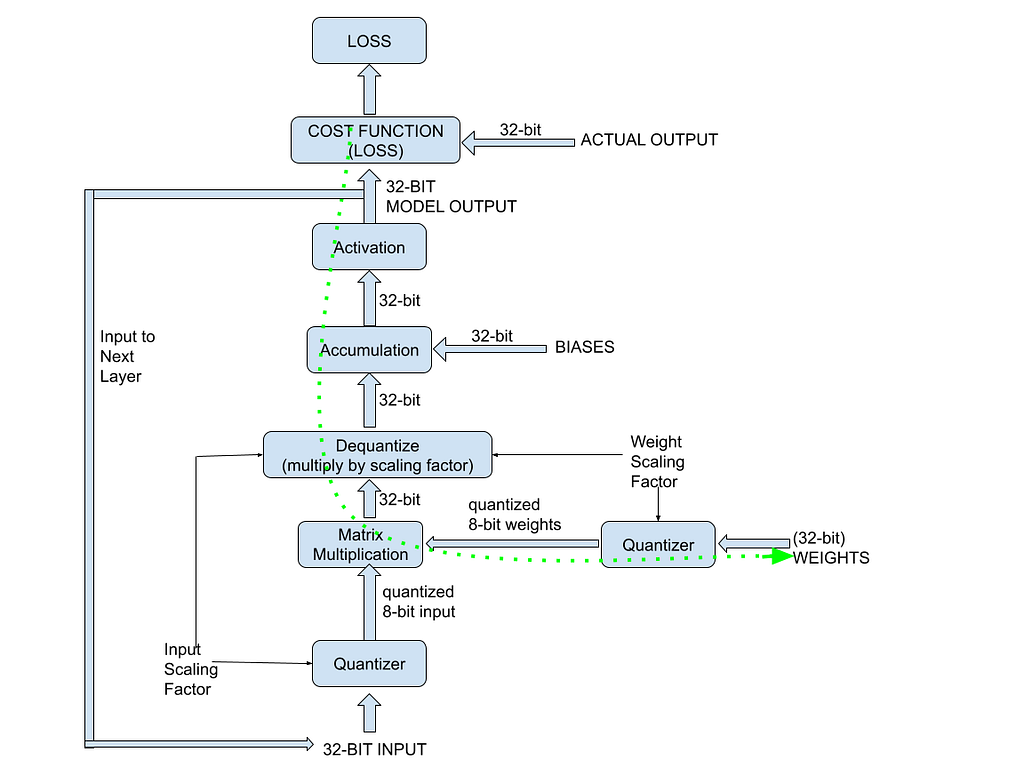
- Run the forward pass (inference) based on a quantized version of the latest shadow weights. This simulates the working of the quantized model. The steps in the forward pass are:
- Quantize the weights and the inputs before matrix-multiplying them.
- Dequantize the output of the convolution (matrix multiplication).
- Add (accumulate) the biases (unquantized) to the output of the convolution.
- Pass the result of the accumulation through the activation function to get the output.
- Compare the model’s output with the expected output and compute the loss of the model. - Backpropagation happens in full precision. This allows for small changes to the model parameters. To perform the backpropagation:
- Compute the gradients in full precision
- Update via gradient descent the full-precision copy of all weights and biases - After training the model, the final quantized version of the weights is exported to use for inference.
QAT is sometimes referred to as “fake quantization” — it just means that the model training happens using the unquantized weights and the quantized weights are used only for the forward pass. The (latest version of the) unquantized weights are quantized during the forward pass.
The flowchart below gives an overview of the QAT process. The dotted green arrow represents the backpropagation path for updating the model weights while training.

The next section explains some of the finer points involved in backpropagating quantized weights.
BackPropagation in Quantization Aware Training
It is important to understand how the gradient computation works when using quantized weights. When the forward pass is modified to include the quantizer function, the backward pass must also be modified to include the gradient of this quantizer function. To refresh neural networks and backprop concepts, refer to Understanding Weight Update in Neural Networks by Simon Palma.
In a regular neural network, given inputs X, weights W, and bias B, the result of the convolution accumulation operation is:

Applying the sigmoid activation function on the convolution gives the model’s output. This is expressed as:

The Cost, C, is a function of the difference between the expected and the actual output. The standard backpropagation process estimates the partial derivative of the cost function, C, with respect to the weights, using the chain rule:

When quantization is involved, the above equation changes to reflect the quantized weight:

Notice that there is an additional term — which is the partial derivative of the quantized weights with respect to the unquantized weights. Look closely at this (last) partial derivative.
Partial derivative of the quantized weights
The quantizer function can simplistically be represented as:

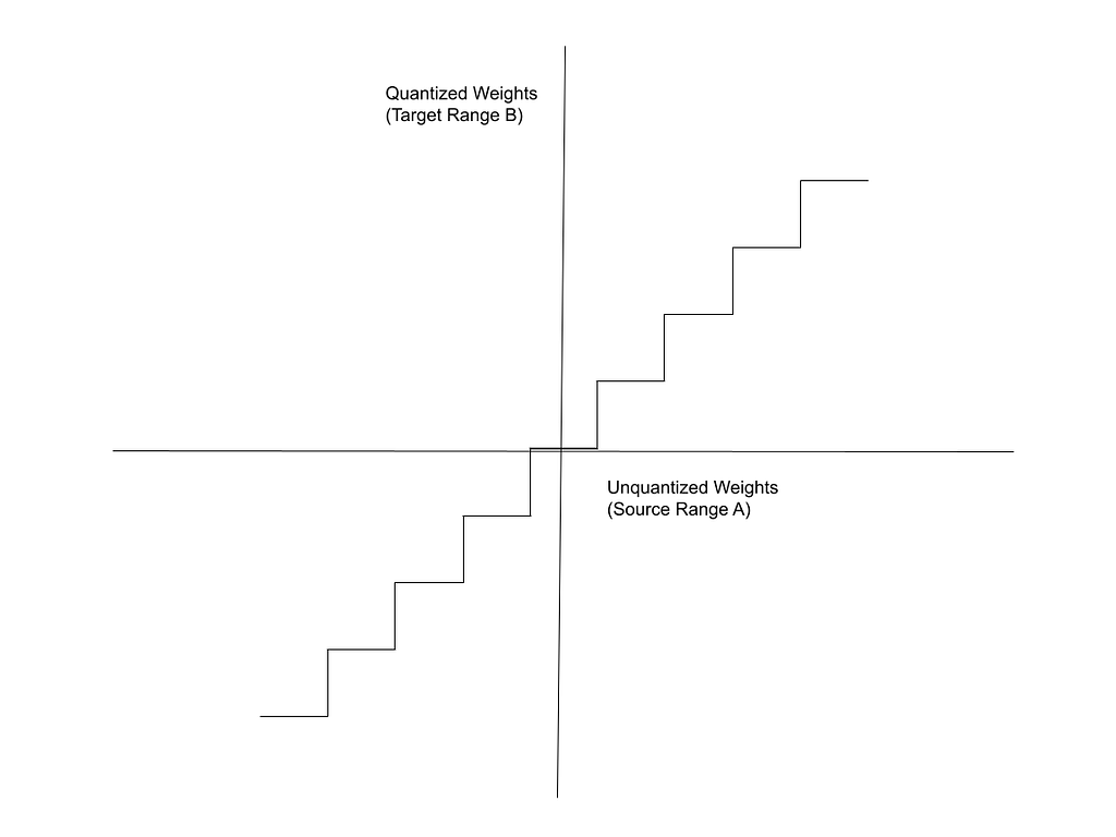
In the expression above, w is the original (unquantized, full-precision) weight, and s is the scaling factor. Recall from Quantizing the Weights of AI Models (or from basic maths) that the graph of the function mapping the floating point weights to the binary weights is a step function, as shown below:

This is the function for which we need the partial derivative. The derivative of the step function is either 0 or undefined — it is undefined at the boundaries between the intervals and 0 everywhere else. To work around this, it is common to use a “Straight-Through Estimator(STE)” for the backprop.
The Straight Through Estimator (STE)
Bengio et al, in their 2013 paper Estimating or Propagating Gradients Through Stochastic Neurons for Conditional Computation, propose the concept of the STE. Huh et al, in their 2023 paper Straightening Out the Straight-Through Estimator: Overcoming Optimization Challenges in Vector Quantized Networks, explain the application of the STE to the derivative of the loss function using the chain rule (Section 2, Equation 7).
The STE assumes that the gradient with respect to the unquantized weight is essentially equal to the gradient with respect to the quantized weight. In other words, it assumes that within the intervals of the Clip function,

Hence, the derivative of the cost function, C, with respect to the unquantized weights is assumed to be equal to the derivative based on the quantized weights.

Thus, the gradient of the Cost is expressed as:

This is how the Straight Through Estimator enables the gradient computation in the backward pass using quantized weights. After estimating the gradients. The weights for the next iteration are updated as usual (alpha in the expression below refers to the learning rate):

The clip function above is to ensure that the updated (unquantized) weights remain within the boundaries, W_min, and W_max.
Conclusion
Quantizing neural network models makes them accessible enough to run on smaller servers and possibly even edge devices. There are two broad approaches to quantizing models, each with its advantages and disadvantages:
- Post-Training Quantization (PTQ): Starting with a high-precision trained model and quantizing it (post-training quantization) to lower-precision.
- Quantization Aware Training (QAT): Applying the quantization during the forward pass of training a model so that the optimization accounts for quantized inference
This article discusses both these approaches but focuses on QAT, which is more effective, especially for modern 1-bit quantized LLMs like BitNet and BitNet b1.58. Since 2021, NVIDIA’s TensorRT has included a Quantization Toolkit to perform both QAT and quantized inference with 8-bit model weights. For a more in-depth discussion of the principles of quantizing neural networks, refer to the 2018 whitepaper Quantizing deep convolutional networks for efficient inference, by Krishnamoorthi.
Quantization encompasses a broad range of techniques that can be applied at different levels of precision, different granularities within a network, and in different ways during the training process. The next article, Different Approaches to Quantization, discusses these varied approaches, which are applied in modern implementations like BinaryBERT, BitNet, and BitNet b1.58.
Quantizing Neural Network Models was originally published in Towards Data Science on Medium, where people are continuing the conversation by highlighting and responding to this story.
from AI in Towards Data Science on Medium https://ift.tt/S5uc90I
via IFTTT


