Datascience in Towards Data Science on Medium,

The Intuition behind Concordance Index — Survival Analysis

11/28/2024 Jesus Santana

The Intuition behind Concordance Index — Survival Analysis

Ranking accuracy versus absolute accuracy

How long would you keep your Gym membership before you decide to cancel it? or Netflix if you are a series fan but busier than usual to allocate 2 hours of your time to your sofa and your TV? Or when to upgrade or replace your smartphone ? What best route to take when considering traffic, road closure, time of the day? or How long until your car needs servicing? These are all regular (but not trivial) questions we face (some of them) in our daily life without thinking too much (or nothing at all) of the thought process we go through on the different factors that influence our next course of action. Surely (or maybe after reading these lines) one would be interested to know what factor or factors could have the greatest influence on the expected time until a given event (from the above or any other for that matter) occurs? In statistics, this is referred as time-to-event-analysis or Survival analysis. And this is the focus of this study.

In Survival Analysis one aims to analyze the time until an event occurs. In this article, I will be employing survival analysis to predict when a registered member is likely to leave (churn), specifically the number of days until a member cancels his/her membership contract. As the variable of interest is the number of days, one key element to explicitly reinforce at this point: the time to event dependent variable is of a continuous type, a variable that can take any value within a certain range. For this, survival analysis is the one to employ.

DATA

This study was conducted using a proprietary dataset provided by a private organization in the tutoring industry. The data includes anonymized records for confidentiality purposes collected over a period of 2 years, namely July 2022 to October 2024. All analyses were conducted in compliance with ethical standards, ensuring data privacy and anonymity. Therefore, to respect the confidentiality of the data provider, any specific organizational details and/or unique identifier details have been omitted.

The final dataset after data pre-processing (i.e. tackling nulls, normalizing to handle outliers, aggregating to remove duplicates and grouping to a sensible level) contains a total of 44,197 records at unique identifier level. A total of 5 columns were input into the model, namely: 1) Age, 2) Number of visits, 3) First visit 4) and Last visit during membership and 5) Tenure. The later representing the number of days holding a membership hence the time-to-event target variable. The visit-based variables are a feature engineered product for this study generated from the original, existing variables and by performing some calculations and aggregation on the raw data for each identifier over the period under analysis. Finally and very importantly, the dataset is ONLY composed of uncensored records. This is, all unique identifiers have experienced the event by the time of the analysis, namely membership cancellation. Therefore there is no censored data in this analysis where individuals survived (did not cancel their membership) beyond their observed duration. This is key when selecting the modelling technique as I will explain next.

Among all different techniques used in survival analysis, three stand out as most commonly used:

Kaplan-Meier Estimator.

• This is a non-parametric model hence no assumptions on the distribution of the data is made.
• KM is not interested on how individual features affect churn thus it does not offer feature-based insights.
• It is widely used for exploratory analysis to assess what the survival curve looks like.
• Very importantly, it does not provide personalized predictions.

Cox Proportional Hazard (PH) Model

• The Cox PH Model is a semi-parametric model so it does not assume any specific distribution of the survival time, making it more flexible for a wider range of data.
• It estimates the hazard function.
• It relies heavily on uncensored as well as censored data to be able to differentiate between individuals “at risk” of experiencing the event versus those who already had the event. Thus, if only uncensored data is analyzed the model assumes all individuals experienced the event yielding bias results thus leading the Cox PH to perform poorly.

AFT Model

• It does not require censor data. Thus, can be used where everyone has experienced the event.
• It directly models the relationship between covariates.
• Used when time-to-event outcomes are of primary interest.
• The model estimate the time-to-event explicitly. Thus, provide direct predictions on the duration until cancellation.

Given the characteristics of the dataset used in this study, I have selected the Accelerated Failure Time (AFT) Model as the most suitable technique. This choice is driven by two key factors: (1) the dataset contains only uncensored data, and (2) the analysis focuses on generating individual-level predictions for each unique identifier.

Now before diving any deeper into the methodology and model output, I will cover some key concepts:

Survival Function: It provides insight into the likelihood of survival over time

Hazard Function: Rate at which the event is taking place at point in time t. It captures how the event is changing over time.

Time-to-event: Refers to the (target) variable capturing the time until an event occurs.

Censoring: Flag referring to those event that have not occurred yet for some of the subjects within the timeframe of the analysis. NOTE: In this piece of work only uncensored data is analyzed, this is the survival time for all the subjects under the study is known.

Concordance Index: A measure of how well the model predicts the relative ordering of survival time. It is a measure of ranking accuracy rather than absolute accuracy that assess the proportion of all pairs of subjects whose predicted survival time align with the actual outcome.

Akaike Information Criterion (AIC): A measure that evaluates the quality of a model penalizing against the number of irrelevant variables used. When comparing several models, the one with the lowest AIC is considered the best.

Next, I will expand on the first two concepts.

In mathematical terms:

The survival function is given by:

where,

T is a random variable representing the time to event — duration until the event occurs.

S(t) is the probability that the event has not yet occurred by time t.

The Hazard function on the other hand is given by:

where,

f(t) is the probability density function (PDF), which describes the rate at which the event occurs at time t.

S(t) is the survival function that describes the probability of surviving beyond time t

As the PDF f(t) can be expressed in terms of the survival function by taking the derivative of S(t) with respect to t:

substituting the derivative of S(t) in the hazard function:

taking the derivative of the Log Survival Function:

from the chain rule of differentiation it follows:

thus, the relationship between the Hazard and Survival function is defined as follow:

the hazard rate captures how quickly the survival probability changes at a specific point in time.

The Hazard function is always non-negative, it can never go below zero. The shape can increase, decrease, stay constant or vary in more complex forms.

Simply put, the hazard function is a measure of the instantaneous risk of experiencing the event at a point in time t. It tells us how likely is the subject to experience the event right then. The survival (rate) function, on the other hand, measures the probability of surviving beyond a given point in time. This is the overall probability of no experiencing the event up to point in time t.

The survival function is always decreasing over time as more and more individuals experience the event. This is illustrated in the below histogram plotting the time-to-event variable: Tenure.

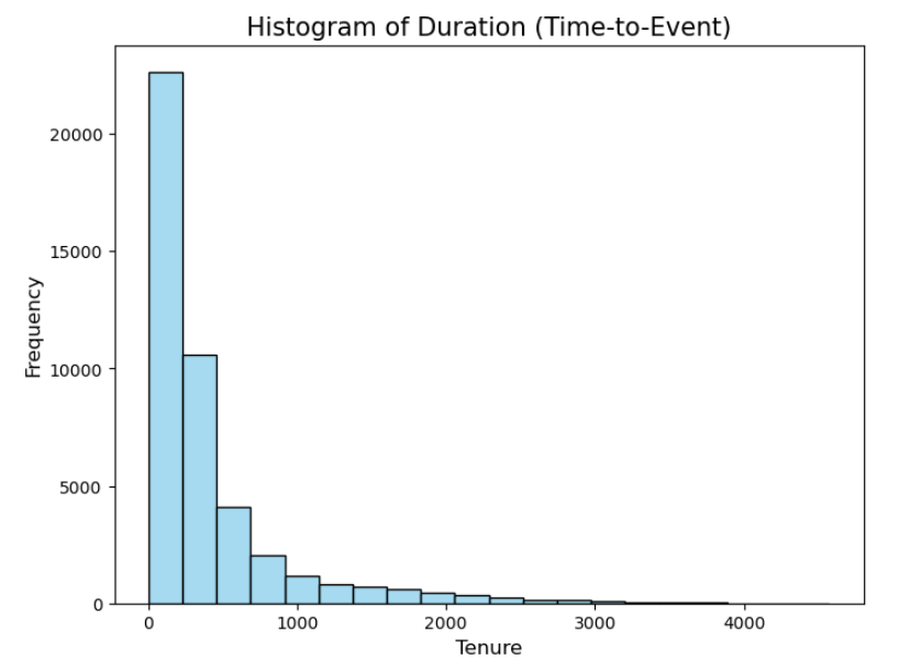
At t=0, no individual has experienced the event (no individual have cancel their membership yet), thus

Eventually all individuals experience the event so the survival function tends to zero (0).

MODEL

For the purposes of this article, I will be focusing on a Multivariate parametric-based model: The Accelerated Failure Time (AFT) model, which explicitly estimate the continuous time-to-event target variable.

Given the AFT Model:

Taking the natural logarithm on both sides of the equation results in:

where,

log(T) is the logarithm of the survival time, namely time-to-event (duration), which as shown by equation (11) is a linear function of the covariates.

X is the vector of covariates

β is the vector of regression coefficients.

and this is very important:

The coefficients β in the model describe how the covariates accelerate or decelerate the event time, namely the survival time. In an AFT Model (the focus of this piece), the coefficients affect directly the survival time (not the hazard function), specifically:

if β > 1 survival time is longer hence leading to a deceleration of the time to event. This is, the member will take longer to terminate his(her) membership (experiencing the event later).

if β < 1 survival time is shorter hence leading to an acceleration of the time to event. This is, the member will terminate his(her) membership earlier (experiencing the event sooner).

finally,

ϵ is the random error term that represents unobserved factors that affect the survival time.

Now, a few explicit points based on the above:

1. this is a Multivariate approach, where the time-to-event (duration) target variable is fit on multiple covariates.
2. a Parametric approach as the model holds an assumption regarding a particular shape of the survival rate distribution.
3. three algorithms sitting under the AFT model umbrella have been implemented. These are:

3.1) Weibull AFT Model

• The model is flexible and can capture different patterns of survival. Supports consistently monotonic increasing/decreasing function. This is: at any two points as defined by the function, the later point is at least as high as the earliest point.
• One does not need to explicitly model the hazard function. The model has two parameters from which the survival function is derived: shape, which determines the shape of the distribution hence helps to determine the skewness of the data and scale which determines the spread of the distribution. This PLUS a regression coefficient related to each covariate. The shape parameter dictates the monotonic behaviors of the hazard function, which in turns affects the behavior of the survival function.
• Right-skewed, left-skewed distributions of the time-to-event target variable are example of these.

3.2) LogNormal AFT Model

• Focuses on modelling the log-transformed of survival time. Logarithm of a random variable whose continuous probability distribution is approximately normally distributed.
• Supports right-skewed distributions of the time-to-event target variable. Allows for non-monotonic hazard functions. Useful when the risk of the event does not follow a simple pattern.
• It does not require to explicitly model the hazard function.
• Two main parameters (plus any regression coefficients): scale and location, the former representing the standard deviation of the log-transformed survival time, the later representing the mean of the log-transformed survival time. This represent the intercept when no covariates are included, otherwise representing the linear combination of these.

3.3) Generalized Gamma AFT Model.

• Good fit for a wide range of survival data patterns. Highly adaptable parametric model that accommodates for the above mentioned shapes as well as more complicated mathematical forms on the survival function.
• It can be used to test if simpler models (i.e. Weibull, logNormal) can be used instead as it encompasses these as special cases.
• It does not require to specify the hazard function.
• It has three parameters apart from the regression coefficient ones: shape, scale and location, the later corresponding to the log of the median of survival time when covariates are not included thus the intercept in the model.

TIP: There is a significant amount of literature on these algorithms that specifically focus on each of these algorithms and their features which I strongly suggest the reader to get an understanding on.

Lastly, the performance of the above algorithms is analyzed focusing on the Concordance Index (yes, the C-Index, our metric of interest) and The Akaike Information Criterion (AIC). These are shown next with the models’ output:

REGRESSION OUTPUTS

Weibull AFT Model

Log Normal AFT Model

Generalized Gamma AFT Model

On the right hand side, the graphs for each predictor are shown: plotting the log accelerated failure rate on the x axis hence their positive/negative (accelerate/decelerate respectively) impact on the survival time. As shown, all models concur across predictors on the direction of the effect on the survival time providing a consistent conclusion about the predictors positive or negative impact. Now, in terms of The Concordance Index and AIC, the LogNormal and Weibull are both shown with the highest C-Index value BUT specifically the LogNormal Model dominating due to a lower AIC. Thus, the LogNormal is selected as the model with the best fit.

Focusing on the LogNormal AFT Model and interpretation of the estimated coefficient for each covariate (coef), in general predictors are all shown with a p-value lower than the conventional threshold 5% significance level hence rejecting the Null Hypothesis and proving to have a statistical significant impact on the survival time. Age is shown with a negative coefficient -0.06 indicating that as age increases, the member is more likely to experience the event sooner hence terminating his(her) membership earlier. This is: each additional year of age represents a 6% decrease in survival time when the later is multiplied by a factor of 0.94 (exp(coef)) hence accelerating the survival time. In contrast, number of visits, first visit since joined and last visit are all shown with a strong positive effect on survival indicating a strong association between, more visits, early engagement and recent engagement increasing survival time.

Now, in terms of The Concordance Index across models (the focus of this analysis), the Generalized Gamma AFT Model is the one with the lowest C-index value hence the model with the weakest predictive accuracy. This is the model with the weakest ability to correctly rank survival times based on the predicted risk scores. This highlights an important aspect about model performance: regardless of the model ability to capture the correct direction of the effect across predictors, this does not necessarily guarantee predictive accuracy, specifically the ability to discriminate across subjects who experience the event sooner versus later as measured by the concordance index. The C-index explicitly evaluates ranking accuracy of the model as opposed to absolute accuracy. This is a fundamental distinction lying at the heart of this analysis, which I will expand next.

CONCORDANCE INDEX (C-INDEX)

A “ranked survival time” refers to the predicted risk scores produced by the model for each individual and used to rank hence discriminate individuals who experience the event earlier when compared to those who experience the event later. Concordance Index is a measure of ranking accuracy rather than absolute accuracy, specifically: the C-index assesses the proportion of all pairs of individuals whose predicted survival time align with the actual outcome. In absolute terms, there is no concern on how precise the model is on predicting the exact number of days it took for the member to cancel its membership, instead how accurate the model ranks individuals when the actual and predicted time it took for a member to cancel its membership align. The below illustrate this:

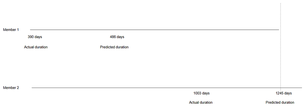
The two instances above are taken from the validation set after the model was trained on the training set and predictions were generated for unseen data. These examples illustrate cases where the predicted survival time (as estimated by the model) exceeds the actual survival time. The horizontal parallel lines represent time.

For Member 1, the actual membership duration was 390 days, whereas the model predicted a duration of 486 days — an overestimation of 96 days. Similarly, Member 2’s actual membership duration was 1,003 days, but the model predicted the membership cancellation to occur 242 days later than it actually did, this is 1,245 days membership duration.

Despite these discrepancies in absolute predictions (and this is important): the model correctly ranked the two members in terms of risk, accurately predicting that Member 1 would cancel their membership before Member 2. This distinction between absolute error and relative ranking is a critical aspect of model evaluation. Consider the following hypothetical scenario:

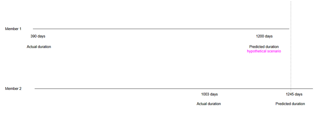
if the model had predicted a membership duration of 1,200 days for Member 1 instead of 486 days, this would not affect the ranking. The model would still predict that Member 1 terminates their membership earlier than Member 2, regardless of the magnitude of the error in the prediction (i.e., the number of days). In survival analysis, any prediction for Member 1 that falls before the dotted line in the graph would maintain the same ranking, classifying this as a concordant pair. This concept is central to calculating the C-index, which measures the proportion of all pairs that are concordant in the dataset.

A couple of hypothetical scenarios are shown below. In each of them, the magnitude of the error increases/decreases, namely the difference between the actual event time and the predicted event time, this is the absolute error. However, the ranking accuracy remains unchanged.

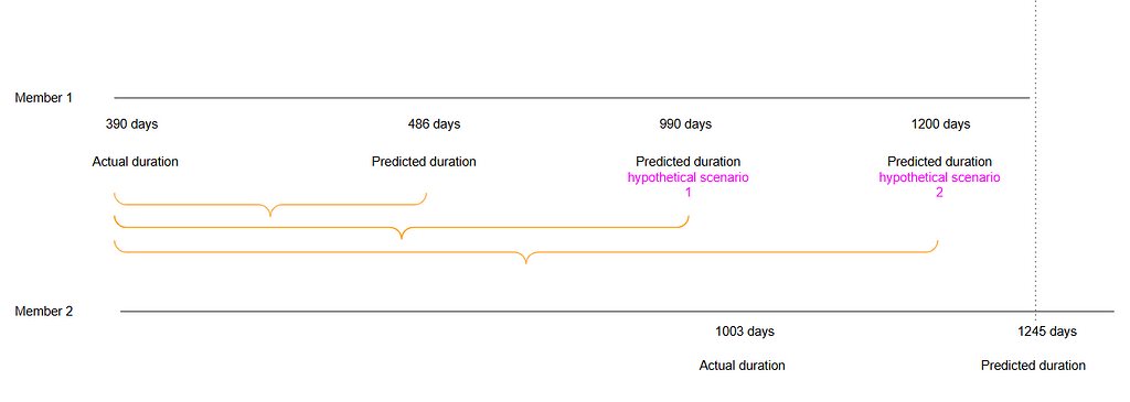
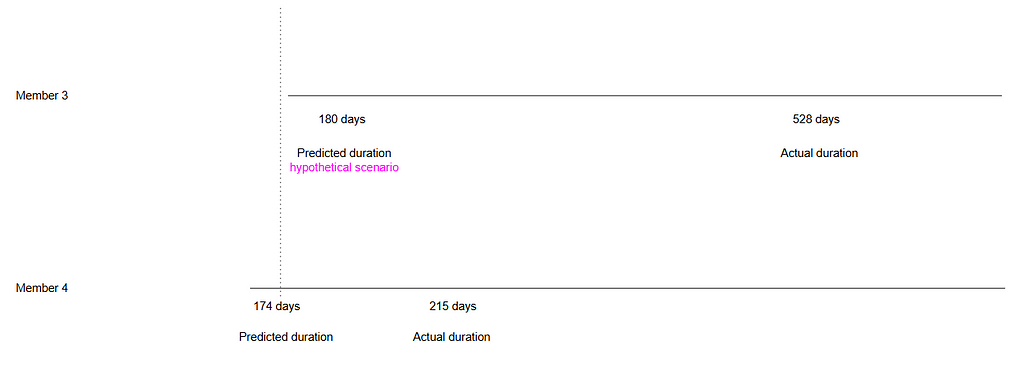
The below are also taken from the validation set BUT for these instances the model predicts the termination of the membership before the actual event occurs. For Member 3, the actual membership duration is 528 days, but the model predicted termination 130 days earlier, namely 398 membership duration. Similarly, for Member 4, the model anticipates the termination of membership before the actual event. In both cases, the model correctly ranks Member 4 to terminate their membership before Member 3.

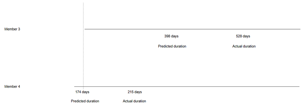
In the hypothetical scenario below, even if the model had predicted the termination 180 days earlier for Member 3, the ranking would remain unchanged. This would still be classified as a concordant pair. We can repeat this analysis multiple times and in 88% of cases, the LogNormal Model will produce this result, as indicated by the concordance index. This is: where the model correctly predicts the relative ordering of the individuals’ survival times.

As everything, the key is to identify when strategically to use survival analysis based on the task at hand. Use cases focusing on ranking individuals employing survival analysis as the most efficient strategy as opposed to focus on reducing the absolute error are:

Customer retention — Businesses rank customers by their likelihood of churning. Survival Analysis would allow to identify the most at risk customers to target retention efforts.

Employee attrition — HR analysis Organizations use survival analysis to predict and rank employees by their likelihood of leaving the company. Similar to the above, allowing to identify most at risk employees. This aiming to improve retention rates and reducing turnover costs.

Healthcare — resource allocation survival models might be used to rank patients based on their risk of adverse outcomes (i.e. disease progression). In here, correctly identifying which patients are at the highest risk and need urgent intervention, allowing to allocate limited resources more effectively is more critical hence more relevant than the exact survival time.

Credit risk — finance Financial institutions employ survival models to rank borrowers based on their risk of default. Thus, they are more concerned on identifying the riskiest customers to make more informed lending decisions rather than focusing on the exact month of default. This would positively guide loan approvals (among others).

On the above, the relative ranking of subjects (e.g., who is at higher or lower risk) directly drives actionable decisions and resource allocation. Absolute error in survival time predictions may not significantly affect the outcomes, as long as the ranking accuracy (C-index) remains high. This demonstrates why models with high C-index can be highly effective, even when their absolute predictions are less precise.

IN SUMMARY

In survival analysis, it is crucial to distinguish between absolute error and ranking accuracy. Absolute error refers to the difference between the predicted and actual event times, in this analysis measured in days. Metrics such as Mean Absolute Error (MAE) or Root Mean Squared Error (RMSE) are used to quantify the magnitude of these discrepancies hence measuring the overall predictive accuracy of the model. However, these metrics do not capture the model’s ability to correctly rank subjects by their likelihood of experiencing the event sooner or later.

Ranking accuracy, on the other hand evaluates how well the model orders subjects based on their predicted risk, regardless of the exact time prediction as illustrated above. This is where the concordance index (C-index) plays a key role. The C-index measures the model’s ability to correctly rank pairs of individuals, with higher values indicating better ranking accuracy. A C-index of 0.88 suggests that the model successfully ranks the risk of membership termination correctly 88% of the time.

Thus, while absolute error provides valuable insights into the precision of time predictions, the C-index focuses on the model’s ability to rank subjects correctly, which is often more important in survival analysis. A model with a high C-index can be highly effective in ranking individuals, even if it has some degree of absolute error, making it a powerful tool for predicting relative risks over time.

---

The Intuition behind Concordance Index — Survival Analysis was originally published in Towards Data Science on Medium, where people are continuing the conversation by highlighting and responding to this story.

from Datascience in Towards Data Science on Medium https://ift.tt/t61icfI
via IFTTT