Tracing the Transformer in Diagrams
What exactly do you put in, what exactly do you get out, and how do you generate text with it?
Last week I was listening to an Acquired episode on Nvidia. The episode talks about transformers: the T in GPT and a candidate for the biggest invention of the 21st century.
Walking down Beacon Street, listening, I was thinking, I understand transformers, right? You mask out tokens during training, you have these attention heads that learn to connect concepts in text, you predict the probability of the next word. I’ve downloaded LLMs from Hugging Face and played with them. I used GPT-3 in the early days before the “chat” part was figured out. At Klaviyo we even built one of the first GPT-powered generative AI features in our subject line assistant. And way back I worked on a grammar checker powered by an older style language model. So maybe.
The transformer was invented by a team at Google working on automated translation, like from English to German. It was introduced to the world in 2017 in the now famous paper Attention Is All You Need. I pulled up the paper and looked at Figure 1:
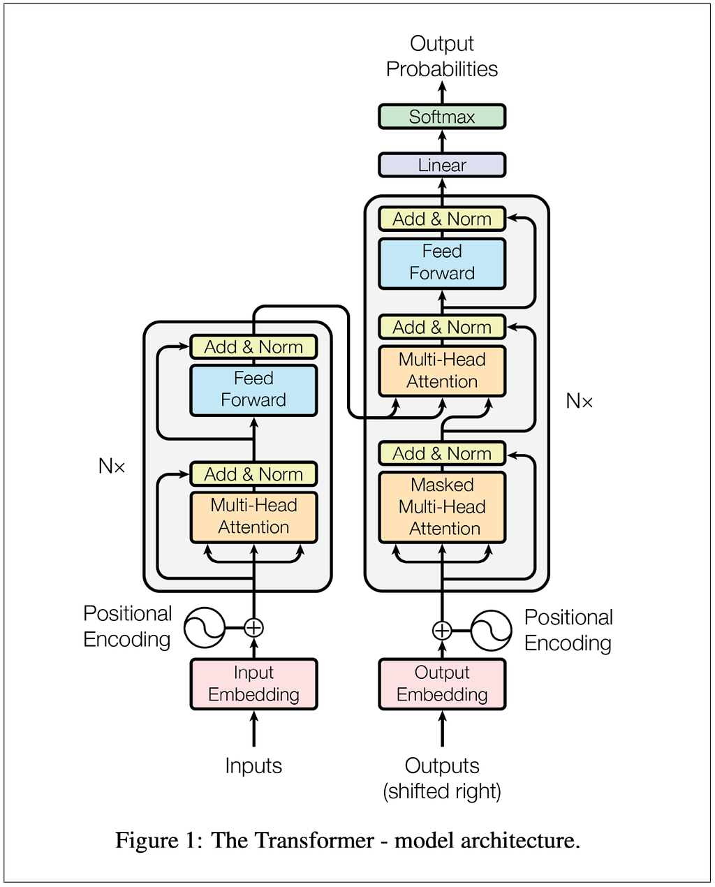
Hmm…if I understood, it was only at the most hand-wavy level. The more I looked at the diagram and read the paper, the more I realized I didn’t get the details. Here are a few questions I wrote down:
- During training, are the inputs the tokenized sentences in English and the outputs the tokenized sentences in German?
- What exactly is each item in a training batch?
- Why do you feed the output into the model and how is “masked multi-head attention” enough to keep it from cheating by learning the outputs from the outputs?
- What exactly is multi-head attention?
- How exactly is loss calculated? It can’t be that it takes a source language sentence, translates the whole thing, and computes the loss, that doesn’t make sense.
- After training, what exactly do you feed in to generate a translation?
- Why are there three arrows going into the multi-head attention blocks?
I’m sure those questions are easy and sound naive to two categories of people. The first is people who were already working with similar models (e.g. RNN, encoder-decoder) to do similar things. They must have instantly understood what the Google team accomplished and how they did it when they read the paper. The second is the many, many more people who realized how important transformers were these last seven years and took the time to learn the details.
Well, I wanted to learn, and I figured the best way was to build the model from scratch. I got lost pretty quickly and instead decided to trace code someone else wrote. I found this terrific notebook that explains the paper and implements the model in PyTorch. I copied the code and trained the model. I kept everything (inputs, batches, vocabulary, dimensions) tiny so that I could trace what was happening at each step. I found that noting the dimensions and the tensors on the diagrams helped me keep things straight. By the time I finished I had pretty good answers to all the questions above, and I’ll get back to answering them after the diagrams.
Here are cleaned up versions of my notes. Everything in this part is for training one single, tiny batch, which means all the tensors in the different diagrams go together.
To keep things easy to follow, and copying an idea from the notebook, we’re going to train the model to copy tokens. For example, once trained, “dog run” should translate to “dog run”.

In other words:

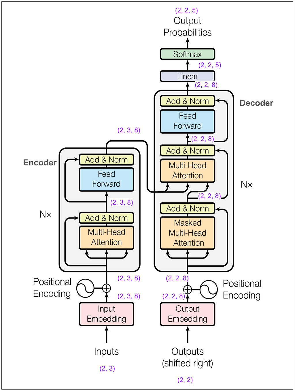
And here’s trying to put into words what the tensor dimensions (shown in purple) on the diagram so far mean:

One of the hyperparameters is d-model and in the base model in the paper it’s 512. In this example I made it 8. This means our embedding vectors have length 8. Here’s the main diagram again with dimensions marked in a bunch of places:
Let’s zoom in on the input to the encoder:
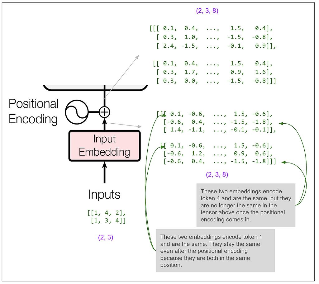

Most of the blocks shown in the diagram (add & norm, feed forward, the final linear transformation) act only on the last dimension (the 8). If that’s all that was happening then the model would only get to use the information in a single position in the sequence to predict a single position. Somewhere it must get to “mix things up” among positions and that magic happens in the multi-head attention blocks.
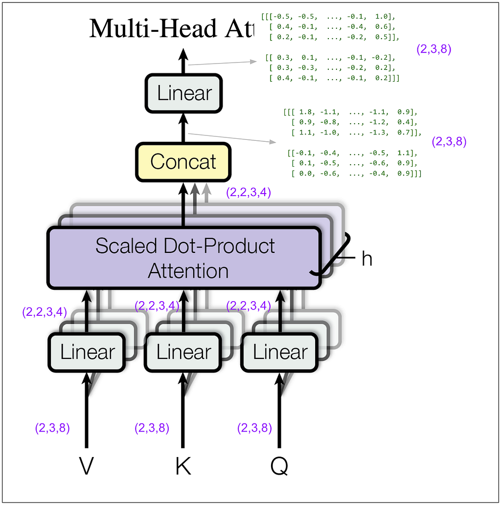
Let’s zoom in on the multi-head attention block within the encoder. For this next diagram, keep in mind that in my example I set the hyperparameter h (number of heads) to 2. (In the base model in the paper it’s 8.)
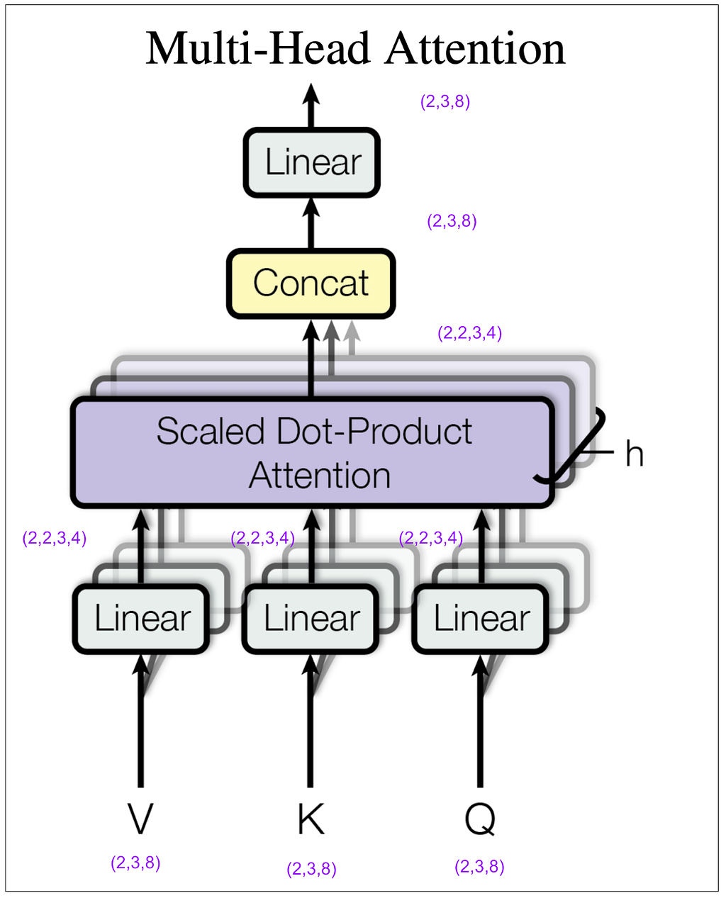
How did (2,3,8) become (2,2,3,4)? We did a linear transformation, then took the result and split it into number of heads (8 / 2 = 4) and rearranged the tensor dimensions so that our second dimension is the head. Let’s look at some actual tensors:
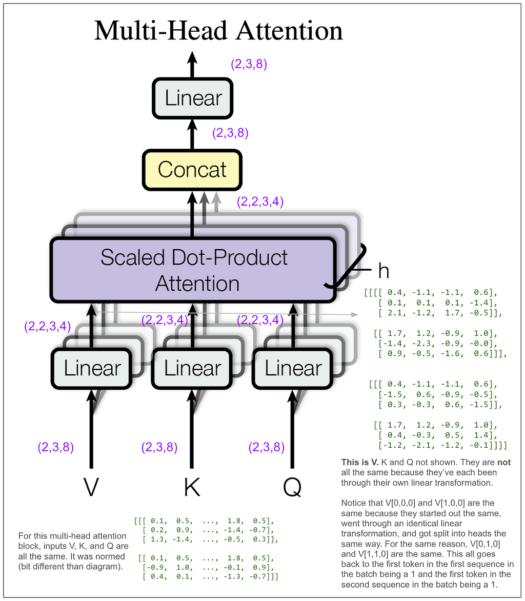
We still haven’t done anything that mixes information among positions. That’s going to happen next in the scaled dot-product attention block. The “4” dimension and the “3” dimension will finally touch.
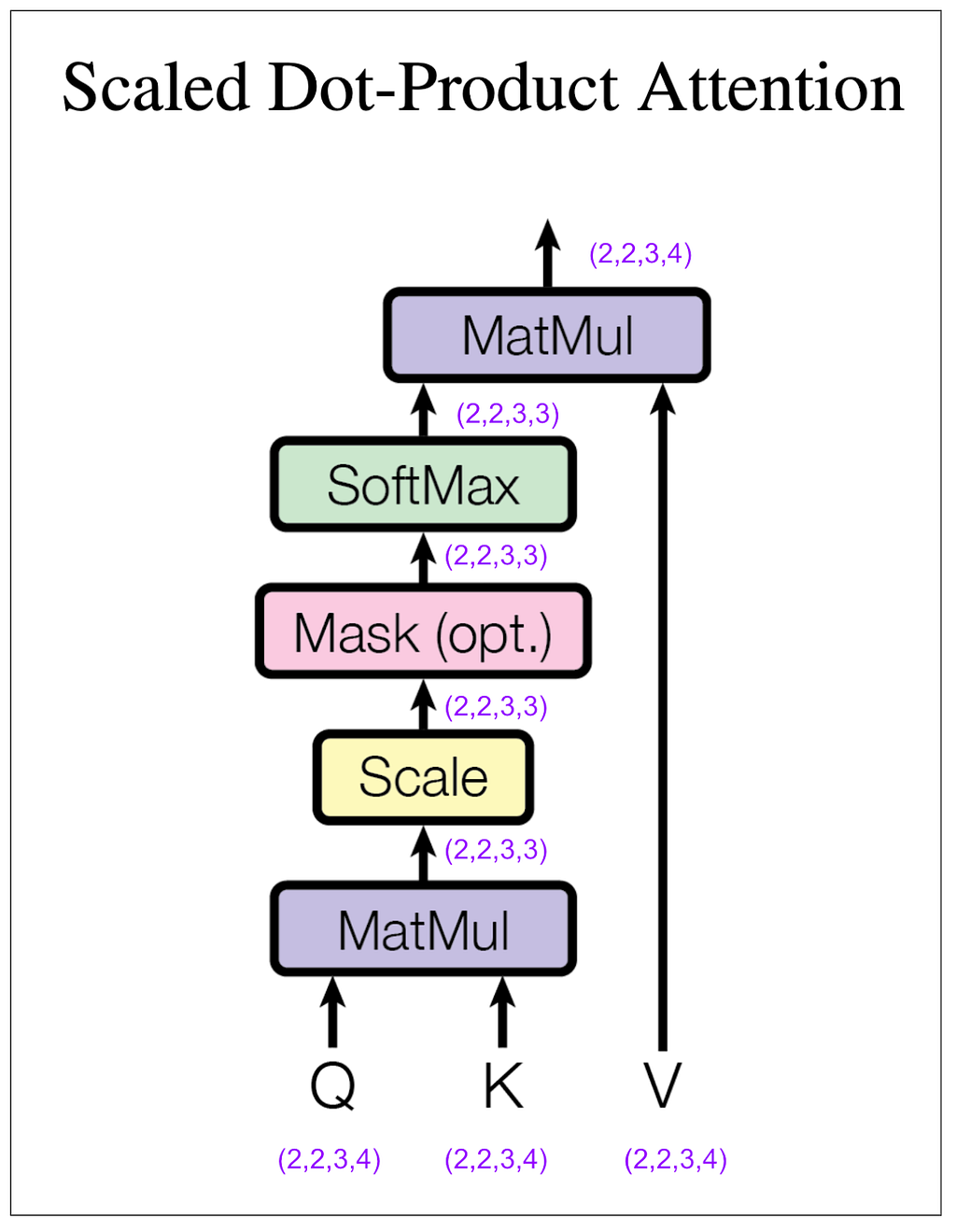
Let’s look at the tensors, but to make it easier to follow, we’ll look only at the first item in the batch and the first head. In other words, Q[0,0], K[0,0], etc. The same thing will be happening to the other three.
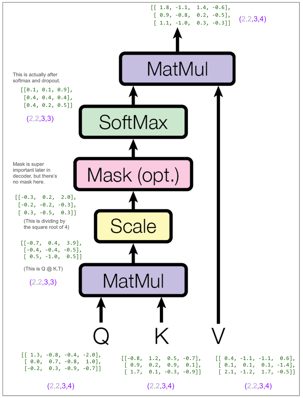
Let’s look at that final matrix multiplication between the output of the softmax and V:
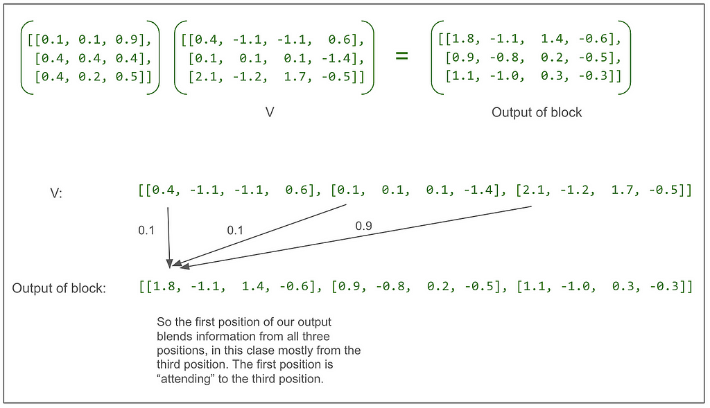
Following from the very beginning, we can see that up until that multiplication, each of the three positions in V going all the way back to our original sentence “<start> dog run” has only been operated on independently. This multiplication blends in information from other positions for the first time.
Going back to the multi-head attention diagram, we can see that the concat puts the output of each head back together so each position is now represented by a vector of length 8. Notice that the 1.8 and the -1.1 in the tensor after concat but before linear match the 1.8 and -1.1 from the first two elements in the vector for the first position of the first head in the first item in the batch from the output of the scaled dot-product attention shown above. (The next two numbers match too but they’re hidden by the ellipses.)
Now let’s zoom back out to the whole encoder:
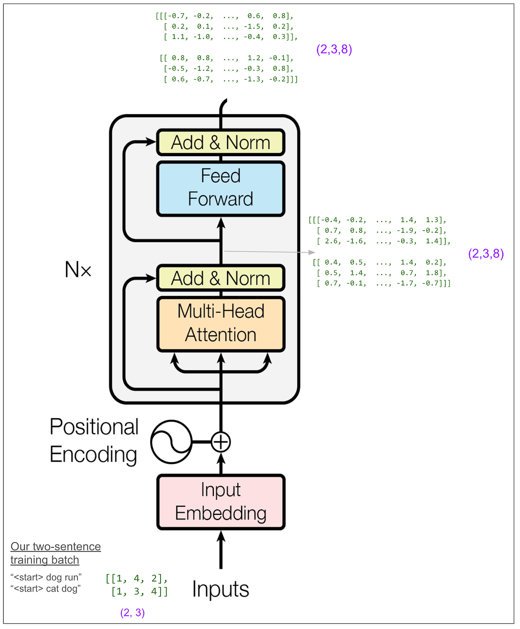
At first I thought I would want to trace the feed forward block in detail. It’s called a “position-wise feed-forward network” in the paper and I thought that meant it might bring information from one position to positions to the right of it. However, it’s not that. “Position-wise” means that it operates independently on each position. It does a linear transform on each position from 8 elements to 32, does ReLU (max of 0 and number), then does another linear transform to get back to 8. (That’s in our small example. In the base model in the paper it goes from 512 to 2048 and then back to 512. There are a lot of parameters here and probably this is where a lot of the learning happens!) The output of the feed forward is back to (2,3,8).
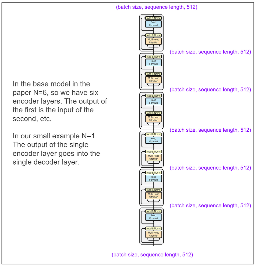
Getting away from our toy model for a second, here’s how the encoder looks in the base model in the paper. It’s very nice that the input and output dimensions match!
Now let’s zoom out all the way so we can look at the decoder.
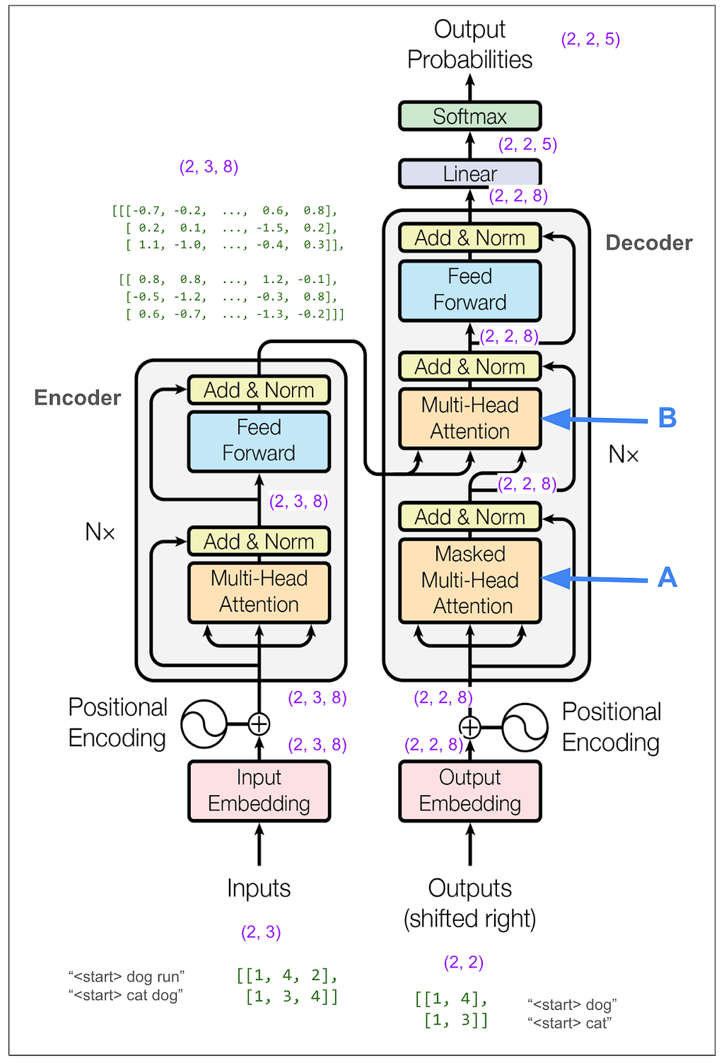
We don’t need to trace most of the decoder side because it’s very similar to what we just looked at on the encoder side. However, the parts I labeled A and B are different. A is different because we do masked multi-head attention. This must be where the magic happens to not “cheat” while training. B we’ll come back to later. But first let’s hide the internal details and keep in mind the big picture of what we want to come out of the decoder.
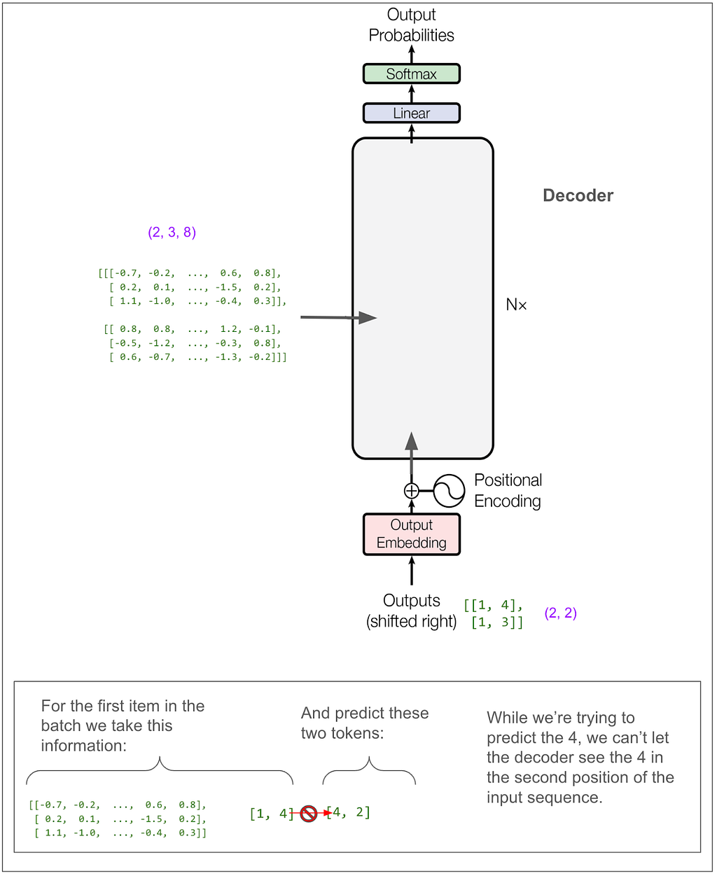
And just to really drive home this point, suppose our English sentence is “she pet the dog” and our translated Pig Latin sentence is “eshay etpay ethay ogday”. If the model has “eshay etpay ethay” and is trying to come up with the next word, “ogday” and “atcay” are both high probability choices. Given the context of the full English sentence of “she pet the dog,” it really should be able to choose “ogday.” However, if the model could see the “ogday” during training, it wouldn’t need to learn how to predict using the context, it would just learn to copy.
Let’s see how the masking does this. We can skip ahead a bit because the first part of A works exactly the same as before where it applies linear transforms and splits things up into heads. The only difference is the dimensions coming into the scaled dot-product attention part are (2,2,2,4) instead of (2,2,3,4) because our original input sequence is of length two. Here’s the scaled dot-product attention part. As we did on the encoder side, we’re looking at only the first item in the batch and the first head.
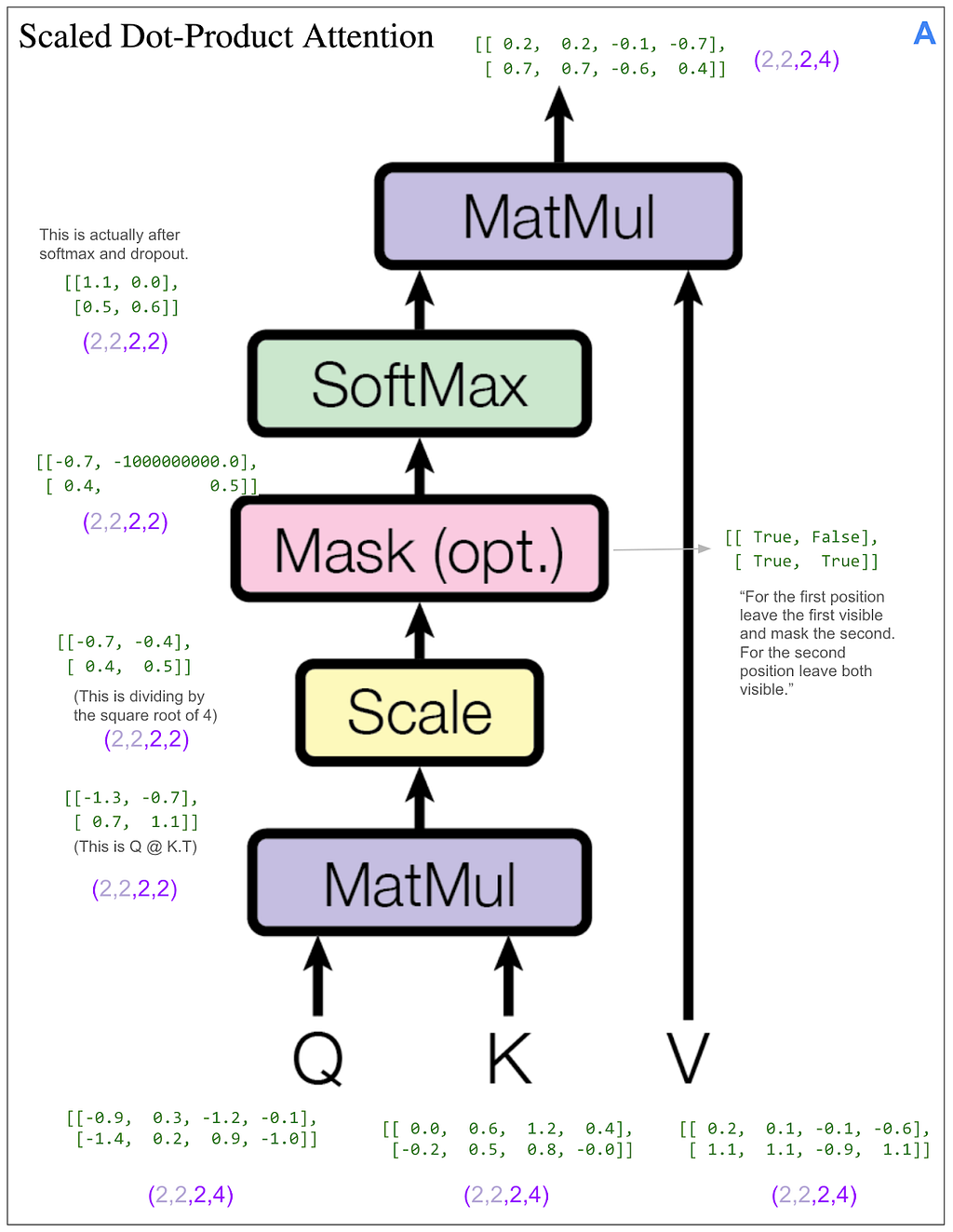
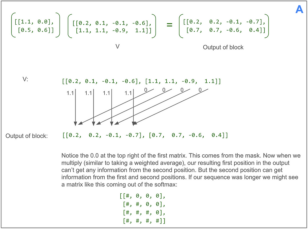
This time we have a mask. Let’s look at the final matrix multiplication between the output of the softmax and V:
Now we’re ready to look at B, the second multi-head attention in the decoder. Unlike the other two multi-head attention blocks, we’re not feeding in three identical tensors, so we need to think about what’s V, what’s K and what’s Q. I labeled the inputs in red. We can see that V and K come from the output of the encoder and have dimension (2,3,8). Q has dimension (2,2,8).
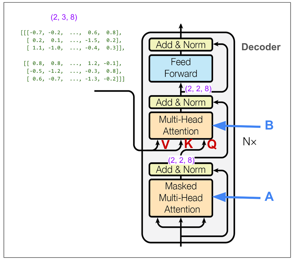
As before, we skip ahead to the scaled dot-product attention part. It makes sense, but is also confusing, that V and K have dimensions (2,2,3,4) — two items in the batch, two heads, three positions, vectors of length four, and Q has dimension (2,2,2,4).

Even though we’re “reading from” the encoder output where the “sequence” length is three, somehow all the matrix math works out and we end up with our desired dimension (2,2,2,4). Let’s look at the final matrix multiplication:
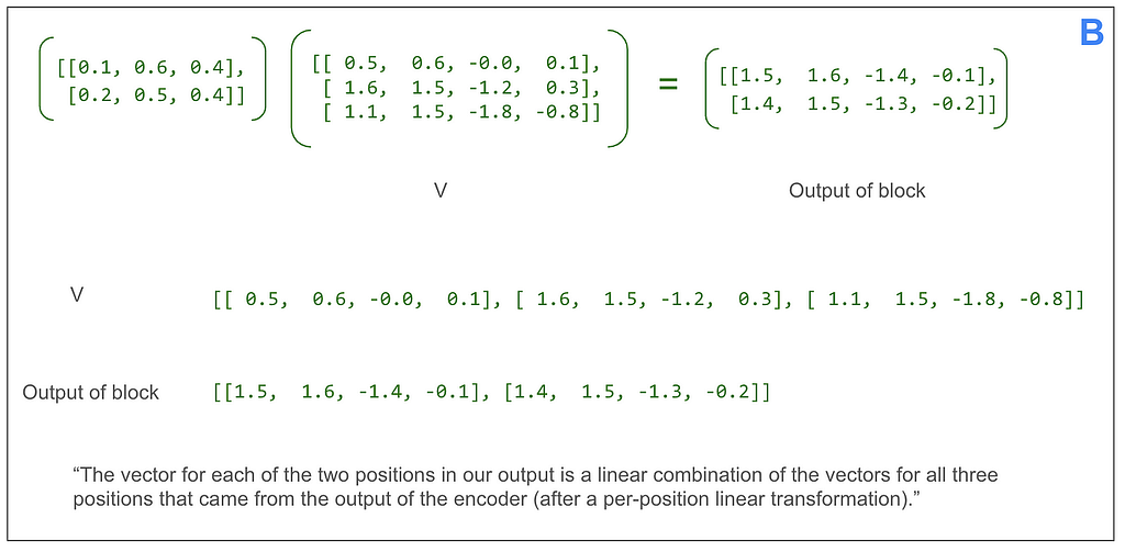
The outputs of each multi-head attention block get added together. Let’s skip ahead to see the output from the decoder and turning that into predictions:
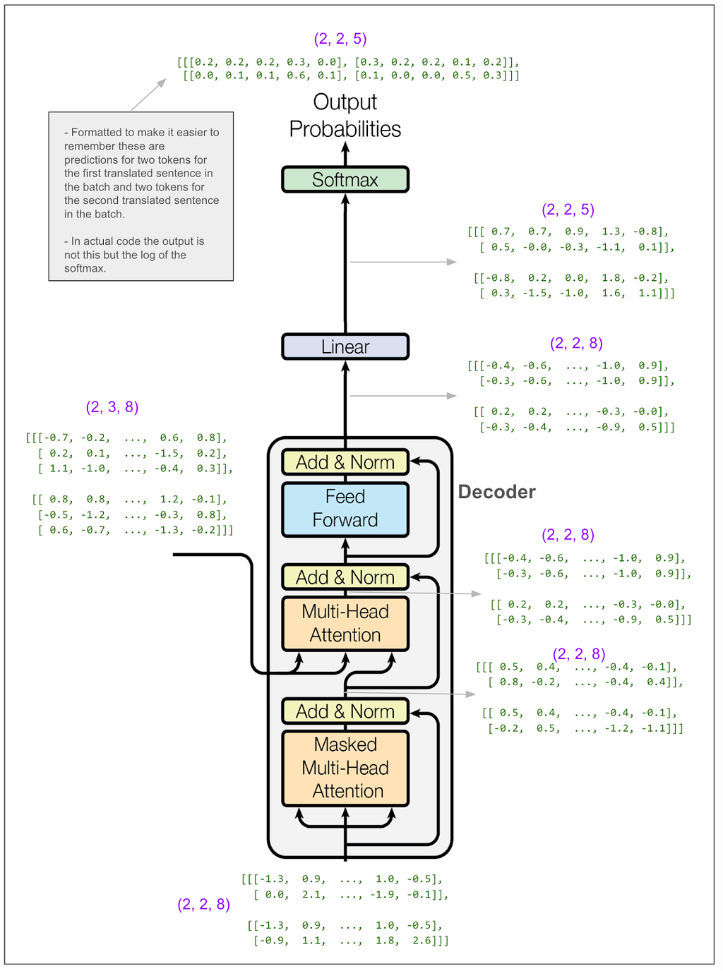
The linear transform takes us from (2,2,8) to (2,2,5). Think about that as reversing the embedding, except that instead of going from a vector of length 8 to the integer identifier for a single token, we go to a probability distribution over our vocabulary of 5 tokens. The numbers in our tiny example make that seem a little funny. In the paper, it’s more like going from a vector of size 512 to a vocabulary of 37,000 when they did English to German.
In a moment we’ll calculate the loss. First, though, even at a glance, you can get a feel for how the model is doing.

It got one token right. No surprise because this is our first training batch and it’s all just random. One nice thing about this diagram is it makes clear that this is a multi-class classification problem. The classes are the vocabulary (5 classes in this case) and, this is what I was confused about before, we make (and score) one prediction per token in the translated sentence, NOT one prediction per sentence. Let’s do the actual loss calculation.
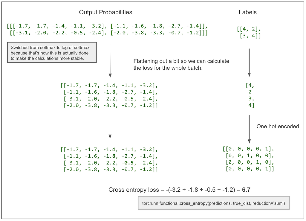
If, for example, the -3.2 became a -2.2, our loss would decrease to 5.7, moving in the desired direction, because we want the model to learn that the correct prediction for that first token is 4.
The diagram above leaves out label smoothing. In the actual paper, the loss calculation smooths labels and uses KL Divergence loss. I think that works out to be the same or simialr to cross entropy when there is no smoothing. Here’s the same diagram as above but with label smoothing.

Let’s also take a quick look at the number of parameters being learned in the encoder and decoder:
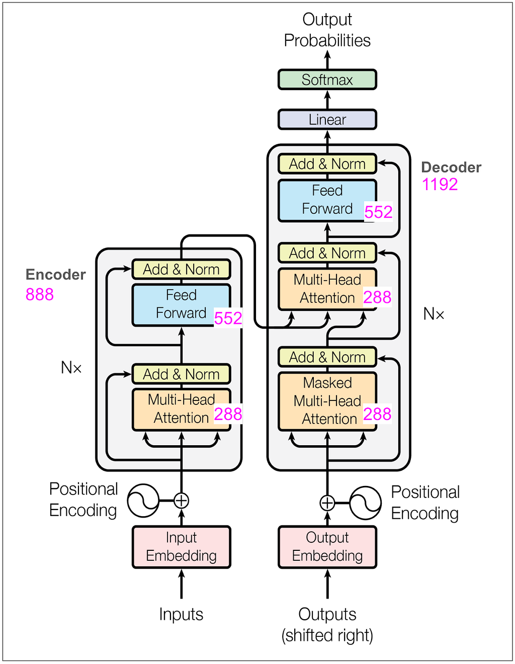
As a sanity check, the feed forward block in our toy model has a linear transformation from 8 to 32 and back to 8 (as explained above) so that’s 8 * 32 (weights) + 32 (bias) + 32 * 8 (weights) + 8 (bias) = 52. Keep in mind that in the base model in the paper, where d-model is 512 and d-ff is 2048 and there are 6 encoders and 6 decoders there will be many more parameters.
Using the trained model
Now let’s see how we put source language text in and get translated text out. I’m still using a toy model here trained to “translate” by coping tokens, but instead of the example above, this one uses a vocabulary of size 11 and d-model is 512. (Above we had vocabulary of size 5 and d-model was 8.)
First let’s do a translation. Then we’ll see how it works.

Step one is to feed the source sentence into the encoder and hold onto its output, which in this case is a tensor with dimensions (1, 10, 512).
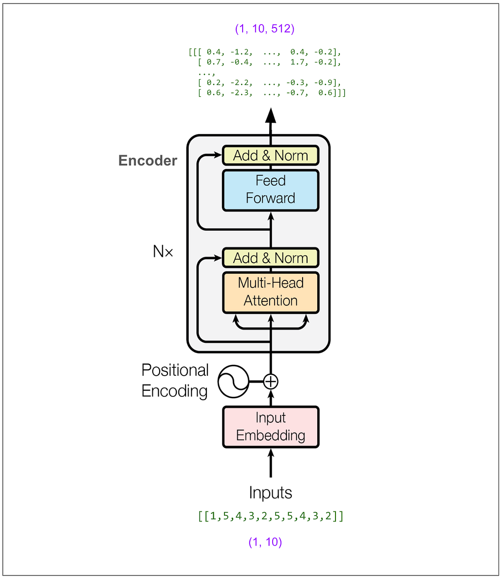
Step two is to feed the first token of the output into the decoder and predict the second token. We know the first token because it’s always <start> = 1.

In the paper, they use beam search with a beam size of 4, which means we would consider the 4 highest probability tokens at this point. To keep things simple I’m going to instead use greedy search. You can think of that as a beam search with a beam size of 1. So, reading off from the top of the diagram, the highest probability token is number 5. (The outputs above are logs of probabilities. The highest probability is still the highest number. In this case that’s -0.0 which is actually -0.004 but I’m only showing one decimal place. The model is really confident that 5 is correct! exp(-0.004) = 99.6%)
Now we feed [1,5] into the decoder. (If we were doing beam search with a beam size of 2, we could instead feed in a batch containing [1,5] and [1,4] which is the next most likely.)
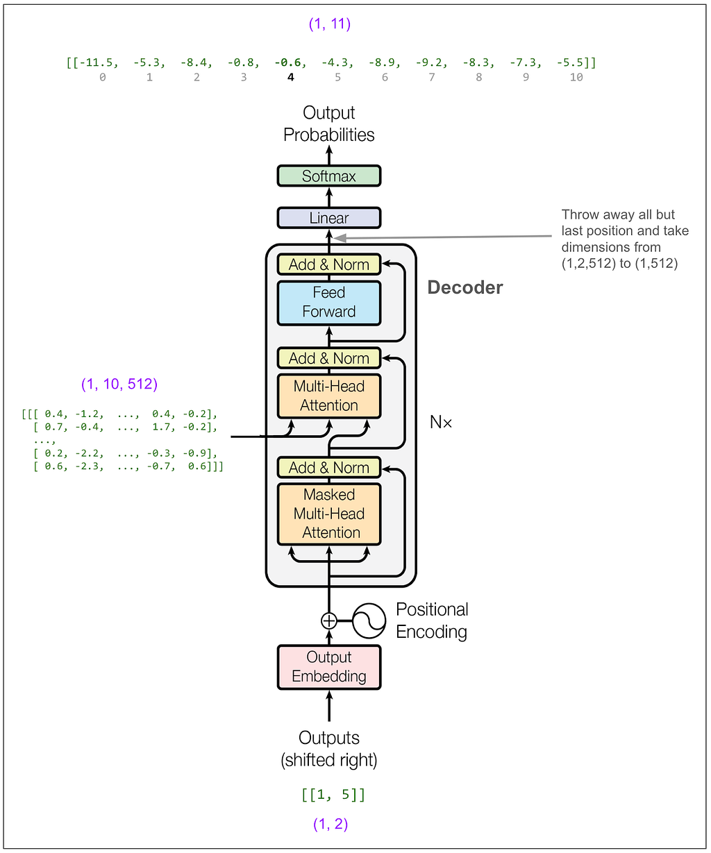
Now we feed [1,5,4]:

And get out 3. And so on until we get a token that indicates the end of the sentence (not present in our example vocabulary) or hit a maximum length.
Circling back to the questions above
Now I can mostly answer my original questions.
During training, are the inputs the tokenized sentences in English and the outputs the tokenized sentences in German?
Yes, more or less.
What exactly is each item in a training batch?
Each item corresponds to one translated sentence pair.
- The “x” of the item has two parts. The first part is all the tokens of the source sentence. The second part is all tokens of the target sentence except for the last one.
- The “y” (label) of the item is all tokens of the target sentence except for the first one. Since the first token for source and target is always <start>, we’re not wasting or losing any training data.
What’s a little subtle is that if this were a classification task where say the model had to take an image and output a class (house, car, rabbit, etc.), we would think of each item in the batch as contributing one “classification” to the loss calculation. Here, however, each item in the batch will contribute (number_of_tokens_in_target_sentence — 1) “classifications” to the loss calculation.
Why do you feed the output into the model and how is “masked multi-head attention” enough to keep it from cheating by learning the outputs from the outputs?
You feed the output so the model can learn to predict the translation based both on the meaning of the source sentence and the words translated so far. Although lots of things are going on in the model, the only time information moves between positions is during the attention steps. Although we do feed the translated sentence into the decoder, the first attention calculation uses a mask to zero out all information from positions beyond the one we’re predicting.
What exactly is multi-head attention?
I probably should have asked what exactly is attention, because that’s the more central concept. Multi-head attention means slicing the vectors up into groups, doing attention on the groups, and then putting the groups back together. For example, if the vectors have size 512 and there are 8 heads, attention will be done independently on 8 groups each containing a full batch of the full positions, each position having a vector of size 64. If you squint, you can see how each head could end up learning to give attention to certain connected concepts as in the famous visualizations showing how a head will learn what word a pronoun references.
How exactly is loss calculated? It can’t be that it takes a source language sentence, translates the whole thing, and computes the loss, that doesn’t make sense.
Right. We’re not translating a full sentence in one go and calculating overall sentence similarity or something like that. Loss is calculated just like in other multi-class classification problems. The classes are the tokens in our vocabulary. The trick is we’re independently predicting a class for every token in the target sentence using only the information we should have at that point. The labels are the actual tokens from our target sentence. Using the predictions and labels we calculate loss using cross entropy. (In reality we “smooth” our labels to account for the fact that they’re notabsolute, a synonym could sometimes work equally well.)
After training, what exactly do you feed in to generate a translation?
You can’t feed something in and have the model spit out the translation in a single evaluation. You need to use the model multiple times. You first feed the source sentence into the encoder part of the model and get an encoded version of the sentence that represents its meaning in some abstract, deep way. Then you feed that encoded information and the start token <start> into the decoder part of the model. That lets you predict the second token in the target sentence. Then you feed in the <start> and second token to predict the third. You repeat this until you have a full translated sentence. (In reality, though, you consider multiple high probability tokens for each position, feed multiple candidate sequences in each time, and pick the final translated sentence based on total probability and a length penalty.)
Why are there three arrows going into the multi-head attention blocks?
I’m guessing three reasons. 1) To show that the second multi-head attention block in the decoder gets some of its input from the encoder and some from the prior block in the decoder. 2) To hint at how the attention algorithm works. 3) To hint that each of the three inputs undergoes its own independent linear transformation before the actual attention happens.
Conclusion
It’s beautiful! I probably wouldn’t think that if it weren’t so incredibly useful. I now get the feeling people must have had when they first saw this thing working. This elegant and trainable model expressible in very little code learned how to translate human languages and beat out complicated machine translations systems built over decades. It’s amazing and clever and unbelievable. You can see how the next step was to say, forget about translated sentence pairs, let’s use this technique on every bit of text on the internet — and LLMs were born!
(I bet have some mistakes above. Please LMK.)
Unless otherwise noted, all images are by author, or contain annotations by the author on figures from Attention Is All You Need.
Tracing the Transformer in Diagrams was originally published in Towards Data Science on Medium, where people are continuing the conversation by highlighting and responding to this story.
from AI in Towards Data Science on Medium https://ift.tt/PYnwvSt
via IFTTT


