Credit Card Fraud Detection with Different Sampling Techniques
How to deal with imbalanced data

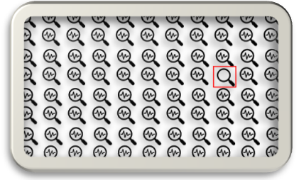
Credit card fraud detection is a plague that all financial institutions are at risk with. In general fraud detection is very challenging because fraudsters are coming up with new and innovative ways of detecting fraud, so it is difficult to find a pattern that we can detect. For example, in the diagram all the icons look the same, but there one icon that is slightly different from the rest and we have pick that one. Can you spot it?

Here it is:

With this background let me provide a plan for today and what you will learn in the context of our use case ‘Credit Card Fraud Detection’:
1. What is data imbalance
2. Possible causes of data Imbalance
3. Why is class imbalance a problem in machine learning
4. Quick Refresher on Random Forest Algorithm
5. Different sampling methods to deal with data Imbalance
6. Comparison of which method works well in our context with a practical Demonstration with Python
7. Business insight on which model to choose and why?
In most cases, because the number of fraudulent transactions is not a huge number, we have to work with a data that typically has a lot of non-frauds compared to Fraud cases. In technical terms such a dataset is called an ‘imbalanced data’. But, it is still essential to detect the fraud cases, because only 1 fraudulent transaction can cause millions of losses to banks/financial institutions. Now, let us delve deeper into what is data imbalance.
We will be considering the credit card fraud dataset from https://www.kaggle.com/mlg-ulb/creditcardfraud (Open Data License).
1. Data Imbalance
Formally this means that the distribution of samples across different classes is unequal. In our case of binary classification problem, there are 2 classes
a) Majority class—the non-fraudulent/genuine transactions
b) Minority class—the fraudulent transactions
In the dataset considered, the class distribution is as follows (Table 1):

As we can observe, the dataset is highly imbalanced with only 0.17% of the observations being in the Fraudulent category.
2. Possible causes of Data Imbalance
There can be 2 main causes of data imbalance:
a) Biased Sampling/Measurement errors: This is due to collection of samples only from one class or from a particular region or samples being mis-classified. This can be resolved by improving the sampling methods
b) Use case/domain characteristic: A more pertinent problem as in our case might be due to the problem of prediction of a rare event, which automatically introduces skewness towards majority class because the occurrence of minor class is practice is not often.
3. Why is class imbalance a problem in machine-learning?
This is a problem because most of the algorithms in machine learning focus on learning from the occurrences that occur frequently i.e. the majority class. This is called the frequency bias. So in cases of imbalanced dataset, these algorithms might not work well. Typically few techniques that will work well are tree based algorithms or anomaly detection algorithms. Traditionally, in fraud detection problems business rule based methods are often used. Tree-based methods work well because a tree creates rule-based hierarchy that can separate both the classes. Decision trees tend to over-fit the data and to eliminate this possibility we will go with an ensemble method. For our use case, we will use the Random Forest Algorithm today.
4. A quick Refresher on Random Forest Algorithm
Random Forest works by building multiple decision tree predictors and the mode of the classes of these individual decision trees is the final selected class or output. It is like voting for the most popular class. For example: If 2 trees predict that Rule 1 indicates Fraud while another tree indicates that Rule 1 predicts Non-fraud, then according to Random forest algorithm the final prediction will be Fraud.
Formal Definition: A random forest is a classifier consisting of a collection of tree-structured classifiers {h(x,Θk ), k=1, …} where the {Θk} are independent identically distributed random vectors and each tree casts a unit vote for the most popular class at input x . (Source)
Each tree depends on a random vector that is independently sampled and all trees have a similar distribution. The generalization error converges as the number of trees increases. In its splitting criteria, Random forest searches for the best feature among a random subset of features and we can also compute variable importance and accordingly do feature selection. The trees can be grown using bagging technique where observations can be random selected (without replacement) from the training set. The other method can be random split selection where a random split is selected from K-best splits at each node.
You can read more about it here
5. Sampling methods to deal with Data Imbalance
We will now illustrate 3 sampling methods that can take care of data imbalance.
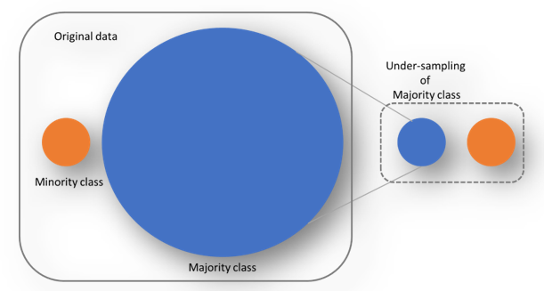
a) Random Under-sampling: Random draws are taken from the non-fraud observations i.e the majority class to match it with the Fraud observations ie the minority class. This means, we are throwing away some information from the dataset which might not be ideal always.

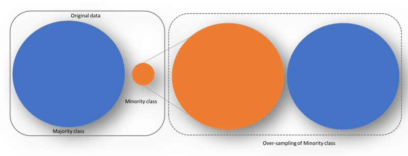
b) Random Over-sampling: In this case, we do exact opposite of under-sampling i.e duplicate the minority class i.e Fraud observations at random to increase the number of the minority class till we get a balanced dataset. Possible limitation is we are creating a lot of duplicates with this method.

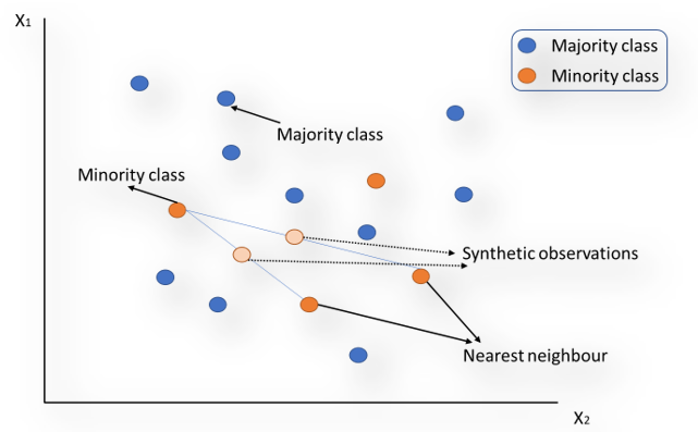
c) SMOTE: (Synthetic Minority Over-sampling technique) is another method that uses synthetic data with KNN instead of using duplicate data. Each minority class example along with their k-nearest neighbours is considered. Then along the line segments that join any/all the minority class examples and k-nearest neighbours synthetic examples are created. This is illustrated in the Fig 3 below:

With only over-sampling, the decision boundary becomes smaller while with SMOTE we can create larger decision regions thereby improving the chance of capturing the minority class better.
One possible limitation is, if the minority class i.e fraudulent observations is spread throughout the data and not distinct then using nearest neighbours to create more fraud cases, introduces noise into the data and this can lead to mis-classification.
6. Quick refresher on Accuracy, Recall, Precision
Some of the metrics that is useful for judging the performance of a model are listed below. These metrics provide a view how well/how accurately the model is able to predict/classify the target variable/s:

· TP (True positive)/TN (True negative) are the cases of correct predictions i.e predicting Fraud cases as Fraud (TP) and predicting non-fraud cases as non-fraud (TN)
· FP (False positive) are those cases that are actually non-fraud but model predicts as Fraud
· FN (False negative) are those cases that are actually fraud but model predicted as non-Fraud
Precision = TP / (TP + FP): Precision measures how accurately model is able to capture fraud i.e out of the total predicted fraud cases, how many actually turned out to be fraud.
Recall = TP/ (TP+FN): Recall measures out of all the actual fraud cases, how many the model could predict correctly as fraud. This is an important metric here.
Accuracy = (TP +TN)/(TP+FP+FN+TN): Measures how many majority as well as minority classes could be correctly classified.
F-score = 2*TP/ (2*TP + FP +FN) = 2* Precision *Recall/ (Precision *Recall) ; This is a balance between precision and recall. Note that precision and recall are inversely related, hence F-score is a good measure to achieve a balance between the two.
7. Comparison of which method works well with a practical demonstration with Python
First, we will train the random forest model with some default features. Please note optimizing the model with feature selection or cross validation has been kept out-of-scope here for sake of simplicity. Post that we train the model using under-sampling, oversampling and then SMOTE. The table below illustrates the confusion matrix along with the precision, recall and accuracy metrics for each method.


a) No sampling result interpretation: Without any sampling we are able to capture 76 fraudulent transactions. Though the overall accuracy is 97%, the recall is 75%. This means that there are quite a few fraudulent transactions that our model is not able to capture.
Below is the code that can be used :
# Training the model
from sklearn.ensemble import RandomForestClassifier
classifier = RandomForestClassifier(n_estimators=10,criterion='entropy', random_state=0)
classifier.fit(x_train,y_train)

# Predict Y on the test set
y_pred = classifier.predict(x_test)

# Obtain the results from the classification report and confusion matrix
from sklearn.metrics import  classification_report, confusion_matrix

print('Classifcation report:\n', classification_report(y_test, y_pred))
conf_mat = confusion_matrix(y_true=y_test, y_pred=y_pred)
print('Confusion matrix:\n', conf_mat)
b) Under-sampling result interpretation: With under-sampling , though the model is able to capture 90 fraud cases with significant improvement in recall, the accuracy and precision falls drastically. This is because the false positives have increased phenomenally and the model is penalizing a lot of genuine transactions.
Under-sampling code snippet:
# This is the pipeline module we need from imblearn
from imblearn.under_sampling import RandomUnderSampler
from imblearn.pipeline import Pipeline

# Define which resampling method and which ML model to use in the pipeline
resampling = RandomUnderSampler()
model = RandomForestClassifier(n_estimators=10,criterion='entropy', random_state=0)

# Define the pipeline,and combine sampling method with the RF model
pipeline = Pipeline([('RandomUnderSampler', resampling), ('RF', model)])

pipeline.fit(x_train, y_train)
predicted = pipeline.predict(x_test)

# Obtain the results from the classification report and confusion matrix
print('Classifcation report:\n', classification_report(y_test, predicted))
conf_mat = confusion_matrix(y_true=y_test, y_pred=predicted)
print('Confusion matrix:\n', conf_mat)
c) Over-sampling result interpretation: Over-sampling method has the highest precision and accuracy and the recall is also good at 81%. We are able to capture 6 more fraud cases and the false positives is pretty low as well. Overall, from the perspective of all the parameters, this model is a good model.
Oversampling code snippet:
# This is the pipeline module we need from imblearn
from imblearn.over_sampling import RandomOverSampler

# Define which resampling method and which ML model to use in the pipeline
resampling = RandomOverSampler()
model = RandomForestClassifier(n_estimators=10,criterion='entropy', random_state=0)

# Define the pipeline,and combine sampling method with the RF model
pipeline = Pipeline([('RandomOverSampler', resampling), ('RF', model)])

pipeline.fit(x_train, y_train)
predicted = pipeline.predict(x_test)

# Obtain the results from the classification report and confusion matrix
print('Classifcation report:\n', classification_report(y_test, predicted))
conf_mat = confusion_matrix(y_true=y_test, y_pred=predicted)
print('Confusion matrix:\n', conf_mat)
d) SMOTE: Smote further improves the over-sampling method with 3 more frauds caught in the net and though false positives increase a bit the recall is pretty healthy at 84%.
SMOTE code snippet:
# This is the pipeline module we need from imblearn

from imblearn.over_sampling import SMOTE


# Define which resampling method and which ML model to use in the pipeline
resampling = SMOTE(sampling_strategy='auto',random_state=0)
model = RandomForestClassifier(n_estimators=10,criterion='entropy', random_state=0)

# Define the pipeline, tell it to combine SMOTE with the RF model
pipeline = Pipeline([('SMOTE', resampling), ('RF', model)])

pipeline.fit(x_train, y_train)
predicted = pipeline.predict(x_test)

# Obtain the results from the classification report and confusion matrix
print('Classifcation report:\n', classification_report(y_test, predicted))
conf_mat = confusion_matrix(y_true=y_test, y_pred=predicted)
print('Confusion matrix:\n', conf_mat)
Summary:
In our use case of fraud detection, the one metric that is most important is recall. This is because the banks/financial institutions are more concerned about catching most of the fraud cases because fraud is expensive and they might lose a lot of money over this. Hence, even if there are few false positives i.e flagging of genuine customers as fraud it might not be too cumbersome because this only means blocking some transactions. However, blocking too many genuine transactions is also not a feasible solution, hence depending on the risk appetite of the financial institution we can go with either simple over-sampling method or SMOTE. We can also tune the parameters of the model, to further enhance the model results using grid search.
For details on the code refer to this link on Github.
References:
[1] Mythili Krishnan, Madhan K. Srinivasan, Credit Card Fraud Detection: An Exploration of Different Sampling Methods to Solve the Class Imbalance Problem (2022), ResearchGate
[1] Bartosz Krawczyk, Learning from imbalanced data: open challenges and future directions (2016), Springer
[2] Nitesh V. Chawla, Kevin W. Bowyer , Lawrence O. Hall and W. Philip Kegelmeyer , SMOTE: Synthetic Minority Over-sampling Technique (2002), Journal of Artificial Intelligence research
[3] Leo Breiman, Random Forests (2001), stat.berkeley.edu
[4] Jeremy Jordan, Learning from imbalanced data (2018)
Credit Card Fraud Detection with Different Sampling Techniques was originally published in Towards Data Science on Medium, where people are continuing the conversation by highlighting and responding to this story.
from Datascience in Towards Data Science on Medium https://ift.tt/3fCnvHp
via IFTTT


