When Averages Lie: Moving Beyond Single-Point Predictions
The Case for Predicting Full Probability Distributions in Decision-Making

Some people like hot coffee, some people like iced coffee, but no one likes lukewarm coffee. Yet, a simple model trained on coffee temperatures might predict that the next coffee served should be… lukewarm. This illustrates a fundamental problem in predictive modeling: focusing on single point estimates (e.g., averages) can lead us to meaningless or even misleading conclusions.
In “The Crystal Ball Fallacy” (Merckel, 2024b), we explored how even a perfect predictive model does not tell us exactly what will happen — it tells us what could happen and how likely each outcome is. In other words, it reveals the true distribution of a random variable. While such a perfect model remains hypothetical, real-world models should still strive to approximate these true distributions.
Yet many predictive models used in the corporate world do something quite different: they focus solely on point estimates — typically the mean or the mode — rather than attempting to capture the full range of possibilities. This is not just a matter of how the predictions are used; this limitation is inherent in the design of many conventional machine learning algorithms. Random forests, generalized linear models (GLM), artificial neural networks (ANNs), and gradient boosting machines, among others, are all designed to predict the expected value (mean) of a distribution when used for regression tasks. In classification problems, while logistic regression and other GLMs naturally attempt to estimate probabilities of class membership, tree-based methods like random forests and gradient boosting produce raw scores that would require additional calibration steps (like isotonic regression or Platt scaling) to be transformed into meaningful probabilities. Yet in practice, this calibration is rarely performed, and even when uncertainty information is available (i.e., the probabilities), it is typically discarded in favor of the single most likely class, i.e., the mode.
This oversimplification is sometimes not just inadequate; it can lead to fundamentally wrong conclusions, much like our lukewarm coffee predictor. A stark example is the Gaussian copula formula used to price collateralized debt obligations (CDOs) before the 2008 financial crisis. By reducing the complex relationships between mortgage defaults to a single correlation number, among other issues, this model catastrophically underestimated the possibility of simultaneous defaults (MacKenzie & Spears, 2014). This systematic underestimation of extreme risks is so pervasive that some investment funds, like Universa Investments advised by Nassim Taleb, incorporate strategies to capitalize on it. They recognize that markets consistently undervalue the probability and impact of extreme events (Patterson, 2023). When we reduce a complex distribution of possible outcomes to a single number, we lose critical information about uncertainty, risk, and potential extreme events that could drastically impact decision-making.
On the other hand, some quantitative trading firms have built their success partly by properly modeling these complex distributions. When asked about Renaissance Technologies’ approach — whose Medallion fund purportedly achieved returns of 66% annually before fees from 1988 to 2018 (Zuckerman, 2019) — founder Jim Simons emphasized that they carefully consider that market risk “is typically not a normal distribution, the tails of a distribution are heavier and the inside is not as heavy” (Simons, 2013, 47:41), highlighting the critical importance of looking beyond simple averages.
Why, then, do we persist in using point estimates despite their clear limitations? The reasons may be both practical and cultural. Predicting distributions is technically more challenging than predicting single values, requiring more sophisticated models and greater computational resources. But more fundamentally, most business processes and tools are simply not designed to handle distributional thinking. You cannot put a probability distribution in a spreadsheet cell, and many decision-making frameworks demand concrete numbers rather than ranges of possibilities. Moreover, as Kahneman (2011) notes in his analysis of human decision-making, we are naturally inclined to think in terms of specific scenarios rather than statistical distributions — our intuitive thinking prefers simple, concrete answers over probabilistic ones.
Let us examine actual housing market data to illustrate potential issues with single-point valuation and possible modeling techniques to capture the full distribution of possible values.
A Deep Dive into Property Pricing
In this section, we use the French Real Estate Transactions (DVF) dataset provided by the French government (gouv.fr, 2024), which contains comprehensive records of property transactions across France. For this analysis, we focus on sale prices, property surface areas, and the number of rooms for the years ranging from 2014 to 2024. Notably, we exclude critical information such as geolocation, as our aim is not to predict house prices but to demonstrate the benefits of predicting distributions over relying solely on single-point estimates.
First, we will go through a fictional — yet most likely à clef — case study where a common machine learning technique is put into action for planning an ambitious real estate operation. Subsequently, we will adopt a critical stance on this case and offer alternatives that many may prefer in order to be better prepared for pulling off the trade.
Case Study: The Homer & Lisa Reliance on AI for Real Estate Trading
Homer and Lisa live in Paris. They expect the family to grow and envisage to sell their two-room flat to fund the acquisition of a four-room property. Given the operational and maintenance costs, and the capacity of their newly acquired state-of-the-art Roomba with all options, they reckoned that 90m² is the perfect surface area for them. They want to estimate how much they need to save/borrow to complement the proceeds from the sale. Homer followed a MOOC on machine learning just before graduating in advanced French literature last year, and immediately found — thanks to his network — a data scientist role at a large reputable traditional firm that was heavily investing in expanding (admittedly from scratch, really) its AI capacity to avoid missing out. Now a Principal Senior Lead Data Scientist, after almost a year of experience, he knows quite a bit! (He even works for a zoo as a side hustle, where his performance has not remained unnoticed — Merckel, 2024a.)
Following some googling, he found the real estate dataset freely provided by the government. He did a bit of cleaning, filtering, and aggregating to obtain the perfect ingredients for his ordinary least squares model (OLS for those in the know). He can now confidently predict prices, in the Paris area, from both the number of rooms and the surface. Their 2-room, 40m², flat is worth 365,116€. And a 4-room, 90m², reaches 804,911€. That is a no-brainer; they must calculate the difference, i.e., 439,795€.
Homer & Lisa: The Ones Playing Darts… Unknowingly!
Do Homer and Lisa need to save/borrow 439,795€? The model certainly suggests so. But is that so?
Perhaps Homer, if only he knew, could have provided confidence intervals? Using OLS, confidence intervals can either be estimated empirically via bootstrapping or analytically using standard error-based methods.
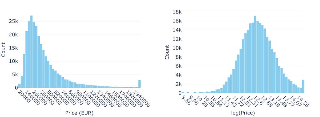
Besides, even before that, he could have looked at the price distribution, and realized the default OLS methods may not be the best choice…

The right-skewed shape with a long tail is hard to miss. For predictive modeling (as opposed to, e.g., explanatory modeling), the primary concern with OLS is not necessarily the normality (and homoscedasticity) of errors but the potential for extreme values in the long tail to disproportionately influence the model — OLS minimizes squared errors, making it sensitive to extreme observations, particularly those that deviate significantly from the Gaussian distribution assumed for the errors.
A Generalized Linear Model (GLM) extends the linear model framework by directly specifying a distribution for the response variable (from the exponential family) and using a “link function” to connect the linear predictor to the mean of that distribution. While linear models assume normally distributed errors and estimate the expected response E(Y) directly through a linear predictor, GLMs allow for different response distributions and transform the relationship between the linear predictor and E(Y) through the link function.
Let us revisit Homer and Lisa’s situation using a simpler but related approach. Rather than implementing a GLM, we can transform the data by taking the natural logarithm of prices before applying a linear model. This implies we are modeling prices as following a log-normal distribution (Figure 1 presents the distribution of prices and the log version). When transforming predictions back to the original scale, we need to account for the bias introduced by the log transformation using Duan’s smearing estimator (Duan, 1983). Using this bias-corrected log-normal model and fitting it on properties around Paris, their current 2-room, 40m² flat is estimated at 337,844€, while their target 4-room, 90m² property would cost around 751,884€, hence a need for an additional 414,040€.
The log-normal model with smearing correction is particularly suitable for this context because it not only reflects multiplicative relationships, such as price increasing proportionally (by a factor) rather than by a fixed amount when the number of rooms or surface area increases, but also properly accounts for the retransformation bias that would otherwise lead to systematic underestimation of prices.
To better understand the uncertainty in these predictions, we can examine their confidence intervals. The 95% bootstrap confidence interval [400,740€ — 418,618€] for the mean price difference means that if we were to repeat this sampling process many times, about 95% of such intervals would contain the true mean price difference. This interval is more reliable in this context than the standard error-based 95% confidence interval because it does not depend on strict parametric assumptions about the model, such as the distribution of errors or the adequacy of the model’s specification. Instead, it captures the observed data’s variability and complexity, accounting for unmodeled factors and potential deviations from idealized assumptions. For instance, our model only considers the number of rooms and surface area, while real estate prices in Paris are influenced by many other factors — proximity to metro stations, architectural style, floor level, building condition, and local neighborhood dynamics, and even broader economic conditions such as prevailing interest rates.
In light of this analysis, the log-normal model provides a new and arguably more realistic point estimate of 414,040€ for the price difference. However, the confidence interval, while statistically rigorous, might not be the most useful for Homer and Lisa’s practical planning needs. Instead, to better understand the full range of possible prices and provide more actionable insights for their planning, we might turn to Bayesian modeling. This approach would allow us to estimate the complete probability distribution of potential price differences, rather than just point estimates and confidence intervals.
The Prior, The Posterior, and The Uncertain
Bayesian modeling offers a more comprehensive approach to understanding uncertainty in predictions. Instead of calculating just a single “best guess” price difference or even a confidence interval, Bayesian methods provide the full probability distribution of possible prices.
The process begins with expressing our “prior beliefs” about property prices — what we consider reasonable based on existing knowledge. In practice, this involves defining prior distributions for the parameters of the model (e.g., the weights of the number of rooms and surface area) and specifying how we believe the data is generated through a likelihood function (which gives us the probability of observing prices given our model parameters). We then incorporate actual sales data (our “evidence”) into the model. By combining these through Bayes’ theorem, we derive the “posterior distribution,” which provides an updated view of the parameters and predictions, reflecting the uncertainty in our estimates given the data. This posterior distribution is what Homer and Lisa would truly find valuable.
Given the right-skewed nature of the price data, a log-normal distribution appears to be a reasonable assumption for the likelihood. This choice should be validated with posterior predictive checks to ensure it adequately captures the data’s characteristics. For the parameters, Half-Gaussian distributions constrained to be positive can reflect our assumption that prices increase with the number of rooms and surface area. The width of these priors reflects the range of possible effects, capturing our uncertainty in how much prices increase with additional rooms or surface area.

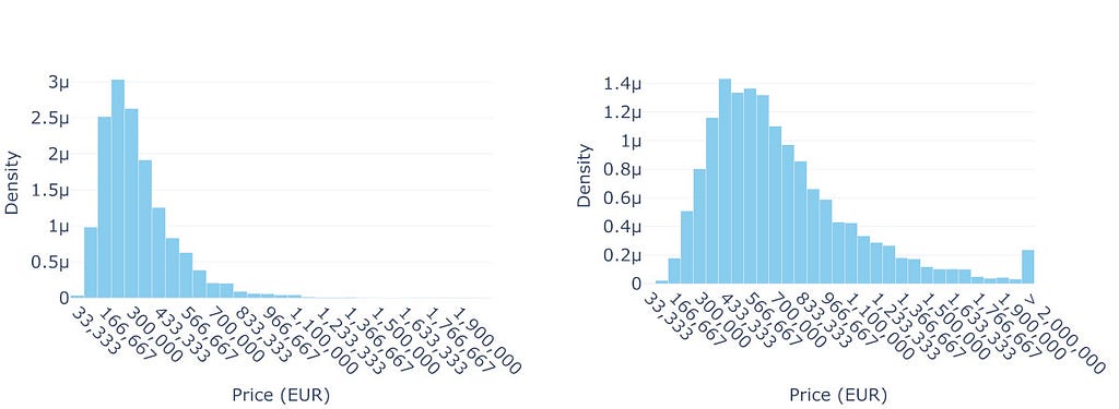
The Bayesian approach provides a stark contrast to our earlier methods. While the OLS and pseudo-GLM (so called because the log-normal distribution is not a member of the exponential family) gave us single predictions with some uncertainty bounds, the Bayesian model reveals complete probability distributions for both properties. Figure 2 illustrates these predicted price distributions, showing not just point estimates but the full range of likely prices for each property type. The overlapping regions between the two distributions reveal that housing prices are not strictly determined by size and room count — unmodeled factors like location quality, building condition, or market timing can sometimes make smaller properties more expensive than larger ones.

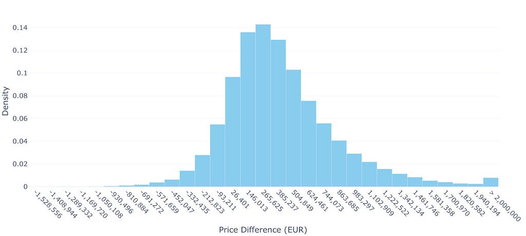
To understand what this means for Homer and Lisa’s situation, we need to estimate the distribution of price differences between the two properties. Using Monte Carlo simulation, we repeatedly draw samples from both predicted distributions and calculate their differences, building up the distribution shown in Figure 3. The results are sobering: while the mean difference suggests they would need to find an additional 405,697€, there is substantial uncertainty around this figure. In fact, approximately 13.4% of the simulated scenarios result in a negative price difference, meaning there is a non-negligible chance they could actually make money on the transaction. However, they should also be prepared for the possibility of needing significantly more money — there is a 25% chance they will need over 611,492€ — and 10% over 956,934€ — extra to make the upgrade.
This more complete picture of uncertainty gives Homer and Lisa a much better foundation for their decision-making than the seemingly precise single numbers provided by our earlier analyses.
Sometimes Less is More: The One With The Raw Data

Rather than relying on sophisticated Bayesian modeling, we can gain clear insights from directly analyzing similar transactions. Looking at properties around Paris, we found 36,265 2-room flats (35–45m²) and 4,145 4-room properties (85–95m²), providing a rich dataset of actual market behavior.
The data shows substantial price variation. Two-room properties have a mean price of 329,080€ and a median price of 323,000€, with 90% of prices falling between 150,000€ and 523,650€. Four-room properties show even wider variation, with a mean price of 812,015€, a median price of 802,090€ and a 90% range from 315,200€ to 1,309,227€.
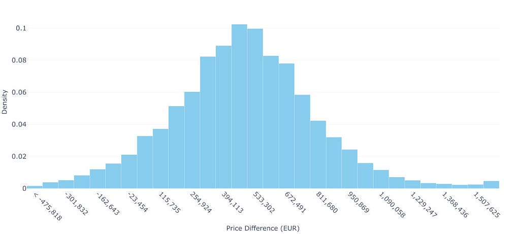
Using Monte Carlo simulation to randomly pair properties, we can estimate what Homer and Lisa might face. The mean price difference is 484,672€ and the median price difference is 480,000€, with the middle 50% of scenarios requiring between 287,488€ and 673,000€. Moreover, in 6.6% of cases, they might even find a 4-room property cheaper than their 2-room sale and make money.
This straightforward approach uses actual transactions rather than model predictions, making no assumptions about price relationships while capturing real market variability. For Homer and Lisa’s planning, the message is clear: while they should prepare for needing around 480,000€, they should be ready for scenarios requiring significantly more or less. Understanding this range of possibilities is crucial for their financial planning.
This simple technique works particularly well here because we have a dense dataset with over 40,000 relevant transactions across our target property categories. However, in many situations relying on predictive modeling, we might face sparse data. In such cases, we would need to interpolate between different data points or extrapolate beyond our available data. This is where Bayesian models are particularly powerful…
Final Remarks
The journey through these analytical approaches — OLS, log-normal modeling, Bayesian analysis, and Monte Carlo simulation — offers more than a range of price predictions. It highlights how we can handle uncertainty in predictive modeling with increasing sophistication. From the deceptively precise OLS estimate (439,795€) to the nuanced log-normal model (414,040€), and finally, to distributional insights provided by Bayesian and Monte Carlo methods (with means of 405,697€ and 484,672€, respectively), each method provides a unique perspective on the same problem.
This progression demonstrates when distributional thinking becomes beneficial. For high-stakes, one-off decisions like Homer and Lisa’s, understanding the full range of possibilities provides a clear advantage. In contrast, repetitive decisions with low individual stakes, like online ad placements, can often rely on simple point estimates. However, in domains where tail risks carry significant consequences — such as portfolio management or major financial planning — modeling the full distribution is not just beneficial but fundamentally wise.
It is important to acknowledge the real-world complexities simplified in this case study. Factors like interest rates, temporal dynamics, transaction costs, and other variables significantly influence real estate pricing. Our objective was not to develop a comprehensive housing price predictor but to illustrate, step-by-step, the progression from a naive single-point estimate to a full distribution.
It is worth noting that, given our primary aim of illustrating this progression — from point estimates to distributional thinking — we deliberately kept our models simple. The OLS and pseudo-GLM implementations were used without interaction terms — and thus without regularization or hyperparameter tuning — and minimal preprocessing was applied. While the high correlation between the number of rooms and surface area is not particularly problematic for predictive modeling in general, it can affect the sampling efficiency of the Markov chain Monte Carlo (MCMC) methods used in our Bayesian models by creating ridges in the posterior distribution that are harder to explore efficiently (indeed, we observed a strong ridge structure with correlation of -0.74 between these parameters, though effective sample sizes remained reasonable at about 50% of total samples, suggesting our inference should be sufficiently stable for our illustrative purposes). For the Bayesian approaches specifically, there is substantial room for improvement through defining more informative priors or the inclusion of additional covariates. While such optimizations might yield somewhat different numerical results, they would likely not fundamentally alter the key insights about the importance of considering full distributions rather than point estimates.
Finally, we must accept that even our understanding of uncertainty is uncertain. The confidence we place in distributional predictions depends on model assumptions and data quality. This “uncertainty about uncertainty” challenges us not only to refine our models but also to communicate their limitations transparently.
Embracing distributional thinking is not merely a technical upgrade — it is a mindset shift. Single-point predictions may feel actionable, but they often provide a false sense of precision, ignoring the inherent variability of outcomes. By considering the full spectrum of possibilities, we equip ourselves to make better-informed decisions and develop strategies that are better prepared for the randomness of the real world.
Sources
References
- Duan, N. (1983). Smearing estimate: A nonparametric retransformation method. Journal of the American Statistical Association, 78(383), 605–610. Available from https://www.jstor.org/stable/2288126.
- Kahneman, D. (2011). Thinking, Fast and Slow. Kindle edition. ASIN B00555X8OA.
- MacKenzie, D., & Spears, T. (2014). ‘The formula that killed Wall Street’: The Gaussian copula and modelling practices in investment banking. Social Studies of Science, 44(3), 393–417. Available from https://www.jstor.org/stable/43284238.
- Patterson, S. (2023). Chaos Kings: How Wall Street Traders Make Billions in the New Age of Crisis. Kindle edition. ASIN B0BSB49L11.
- Zuckerman, G. (2019). The Man Who Solved the Market: How Jim Simons Launched the Quant Revolution. Kindle edition. ASIN B07NLFC63Y.
Notes
- gouv.fr (2024). Demandes de valeurs foncières (DVF), Retrieved from https://www.data.gouv.fr/fr/datasets/5c4ae55a634f4117716d5656/.
- Merckel, L. (2024a). Data-Driven or Data-Derailed? Lessons from the Hello-World Classifier. Retrieved from https://619.io/blog/2024/11/28/data-driven-or-data-derailed/.
- Merckel, L. (2024b). The Crystal Ball Fallacy: What Perfect Predictive Models Really Mean. Retrieved from https://619.io/blog/2024/12/03/the-crystal-ball-fallacy/.
- Simons, J. H. (2013). Mathematics, Common Sense, and Good Luck: My Life and Careers. Video lecture. YouTube. https://www.youtube.com/watch?v=SVdTF4_QrTM.
Art and text by Loic Merckel. Licensed under CC BY 4.0. Originally published on 619.io. For discussions or engagement, feel free to refer to the LinkedIn version or Medium version. Otherwise, attribute the original source when sharing or reusing.
When Averages Lie: Moving Beyond Single-Point Predictions was originally published in Towards Data Science on Medium, where people are continuing the conversation by highlighting and responding to this story.
from Datascience in Towards Data Science on Medium https://ift.tt/MSvCO4f
via IFTTT


