How to Tell Among Two Regression Models with Statistical Significance
Diving into the F-test for nested models with algorithms, examples and code
Introduction
When analyzing data, one often needs to compare two regression models to determine which one fits best to a piece of data. Often, one model is a simpler version of a more complex model that includes additional parameters. However, more parameters do not always guarantee that a more complex model is actually better, as they could simply overfit the data.
To determine whether the added complexity is statistically significant, we can use what’s called the F-test for nested models. This statistical technique evaluates whether the reduction in the Residual Sum of Squares (RSS) due to the additional parameters is meaningful or just due to chance.
In this article I explain the F-test for nested models and then I present a step-by-step algorithm, demonstrate its implementation using pseudocode, and provide Matlab code that you can run right away or re-implement in your favorite system (here I chose Matlab because it gave me quick access to statistics and fitting functions, on which I didn’t want to spend time). Throughout the article we will see examples of the F-test for nested models at work in a couple of settings including some examples I built into the example Matlab code.
The F-test for Nested Models
What Are Nested Models?
Two models are nested if the simpler model is a special case of the more complex model. In other words, the simpler model can be obtained from the complex model by setting some parameters to zero or fixing them; or simply just by removing one or more terms.
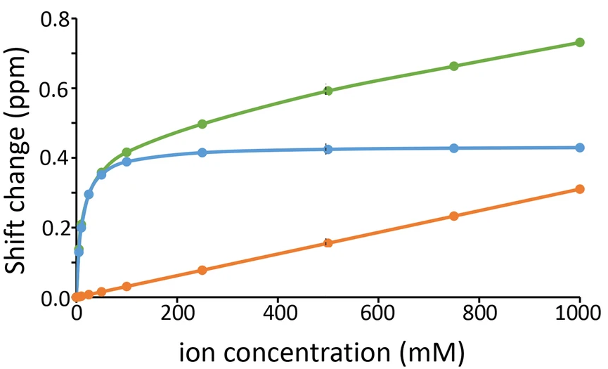
For example, in this paper the authors followed a spectroscopic observable (from an NMR experiment, learn about it here) vs. concentration, and they found that most of the times the dependence is linear but in some cases it is a combination of linear plus hyperbolic saturation with a binding-like shape:

This means one can fit either a simple model which looks just like a linear regression:

Or a more complex that extends the simpler one by adding the binding term:

In this case, the simple model has two parameters, and the complex model has two more parameters inside a term that simply extends from the linear one. And if you remove the hyperbolic binding term, the complex model reduces to the simpler model, making these two models nested.
How the F-test Works
The F-test compares the Residual Sum of Squares (RSS) of two models to test if the reduction in RSS achieved by the complex model is statistically significant. The RSS measures the total squared differences between the observed data and the fitted model, and we compare the RSS for each model using an F-statistic (Snedecor’s F) computed as:

where…
- RSS 1 and RSS 2 are the RSS for the simpler (1) and complex (2) models (note that subtracting in this order ensures that the difference is equal to or larger than zero)
- p2 and p1 are the numbers of parameters in each model, here 4 and 2 respectively.
- n is the number of points we are fitting.
The F-statistic follows an F-distribution with (numerator) and (denominator) degrees of freedom, that we can look up in a table or get with a function in most programs and libraries for statistics. From this, a p-value can be obtained to determine statistical significance.
Interpreting the F-test
Nothing out of the ordinary. If the p-value < some threshold (e.g., 0.05), the complex model fits the data significantly better than the simpler model. Otherwise, the simpler model is sufficient.
By the way, at this point you might be interested in checking this article about statistical significance:
Rethinking Statistical Significance
Algorithm for Model Comparison
The step-by-step algorithm for comparing two nested models is as follows:
- Define the two models: Simple model with fewer parameters; complex model with additional parameters, that includes the simple model under some circumstance.
- Fit both models to the data to estimate their parameters and compute their RSSs.
- Compute the F-statistic from the RSS values, as indicated.
- Calculate the p-value using the F-distribution and check significance.
Pseudocode
The following pseudocode outlines the logic for comparing two nested models. I implemented this piece of pseudocode following the example shown above coming from that paper.
Input: x (independent variable), y (dependent variable)
Output: Parameters of both models, p-value, and decision

1. Define Simple Model: y_simple = a*x + h
2. Define Complex Model: y_complex = a*x + h + c*x / (d + x)
3. Fit the Simple Model to the data (x, y) to find parameters and compute RSS1.
4. Fit the Complex Model to the data (x, y) to find parameters and compute RSS2.
5. Compute F-statistic:
      F = ((RSS1 - RSS2) / (p2 - p1)) / (RSS2 / (n - p2))
6. Compute p-value from the F-distribution with (p2 - p1, n - p2) degrees of freedom.
7. If p-value < alpha (e.g., 0.05):
       Print "The complex model is significantly better."
   Else:
       Print "The simpler model is sufficient."
8. Plot the data with both model fits for visualization (optional).
MATLAB Code Implementation
I know Matlab isn’t popular around here, but in this specific case it was convenient for the problem I was working on because it has all the libraries and functions I need for statistics and fitting without the need to do any special calls or sourcing libraries. This way, I can focus on the F-test itself.
But of course, feel free to adapt to your preferred programming language, statistics package or libraries!
Here is the full Matlab implementation of the algorithm, in the form of a function called compare_models that, well.. does just that (together with a function that takes care of the fits):
function compare_models(x, y)
    % Fit Simple Model: y = a*x + h
    simple_model = @(b, x) b(1)*x + b(2);
    b0_simple = [1; 0];
    [params_simple, RSS1] = fit_model(simple_model, b0_simple, x, y);

    % Fit Complex Model: y = a*x + h + c*x / (d + x)
    complex_model = @(b, x) b(1)*x + b(2) + b(3)*x ./ (b(4) + x);
    b0_complex = [1; 0; 1; 1];
    [params_complex, RSS2] = fit_model(complex_model, b0_complex, x, y);

    % Degrees of freedom
    n = length(y);
    p1 = 2; p2 = 4;
    df1 = p2 - p1; df2 = n - p2;

    % Compute F-statistic and p-value
    F = ((RSS1 - RSS2) / df1) / (RSS2 / df2);
    p_value = 1 - fcdf(F, df1, df2);

    % Print results
    fprintf('Simple Model Parameters: a = %.4f, h = %.4f\n', params_simple(1), params_simple(2));
    fprintf('Complex Model Parameters: a = %.4f, h = %.4f, c = %.4f, d = %.4f\n', ...
        params_complex(1), params_complex(2), params_complex(3), params_complex(4));
    fprintf('F-statistic: %.4f, p-value: %.4e\n', F, p_value);

    % Decision
    if p_value < 0.05
        fprintf('The complex model is significantly better.\n');
    else
        fprintf('The simpler model is sufficient.\n');
    end
end

%% Auxiliary function that runs the least-squares fitting procedure
function [params, RSS] = fit_model(model, b0, x, y)
    opts = optimset('Display', 'off');
    [params, ~] = lsqcurvefit(model, b0, x, y, [], [], opts);
    residuals = y - model(params, x);
    RSS = sum(residuals.^2);
end
Example Usage
We can prepare some example data in two vectors, and then just call the function passing the two arguments:
x = [0, 1, 2, 3, 4, 5, 6, 7, 8, 9, 10]';
y = [0, 2.1, 4.1, 6.3, 8.1, 10.2, 12.0, 13.9, 15.1, 17.2, 19.0]';

compare_models(x, y);
The output will look something like this:
Simple Model Parameters: a = 2.1234, h = 1.2345
Complex Model Parameters: a = 1.9876, h = 1.4567, c = 5.6789, d = 2.3456
F-statistic: 12.3456, p-value: 1.23e-03
The complex model is significantly better.
Some more examples
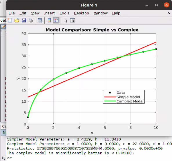
We can easily create Matlab code that will not only return whether the complex model is significantly better but also show a plot so that we as experts can inspect the situation critically:

Here’s the full code for that exact example, where I don’t show the functions defined earlier in order to make it all more compact and straightforward:
clc
clear
close all

% Example data
x = [0, 1, 2, 3, 4, 5, 6, 7, 8, 9, 10]';

y = 1.*x + 3 + 22.*x./(x+1);

% Plot original data
figure;
plot(x, y, 'k.', 'MarkerSize', 15); % Original data in black
hold on;
xlabel('x');
ylabel('y');
title('Model Comparison: Simple vs Complex');
grid on;

% Run the comparison
[params_simple, params_complex, p_value, is_significant] = compare_fits(x, y);

% Generate fitted data for the two models
x_fit = linspace(min(x), max(x), 100)'; % Fine grid for smooth curve

% Simple model: y = a*x + h
y_simple = params_simple(1) * x_fit + params_simple(2);

% Complex model: y = a*x + h + c*x/(d+x)
y_complex = params_complex(1) * x_fit + params_complex(2) + ...
            params_complex(3) * x_fit ./ (params_complex(4) + x_fit);

% Overlay the fitted models
plot(x_fit, y_simple, 'r-', 'LineWidth', 2, 'DisplayName', 'Simple Model: y = a*x + h'); % Red curve
plot(x_fit, y_complex, 'g-', 'LineWidth', 2, 'DisplayName', 'Complex Model: y = a*x + h + c*x/(d+x)'); % Green curve

% Add legend
legend('Data', 'Simple Model', 'Complex Model', 'Location', 'best');
hold off;
Screening Through Fits
What we have seen here was presented as a way to tell, with statistical significance, whether a model fits better than another, simpler one. However, there’s a much more interesting “secondary” application stemming from this “direct” application. Indeed it was this secondary application what prompted me to work on this problem: You can run fits automatically on various (x, y) vectors to detect trends automatically.
For instance, in the example I started this post with, one could run the fits and F-tests on various sets of concentrations and signals to automatically determine in which cases one can detect binding in the form of statistically significant fits to the more complex model.
One can easily edit the Matlab code I provided above to run through various (x, y) sets and print flags each time the more complex model fits statistically better, possibly also plotting the data and fits so that the user can inspect the results and judge the conclusion based on expertise:

Conclusion
We went here through the F-test for nested models, a powerful statistical technique that compares two regression models and determines if the added complexity of the more complex model is “statistically justified”. By implementing this method, you ensure that your model selection is grounded in statistical evidence rather than subjective preference.
If you liked this, here are other deep hands-on explanations that I wrote and you may enjoy or find useful:
- The power and simplicity of propagating errors with Monte Carlo simulations
- The Definitive Guide to Principal Components Analysis
- A framework to evaluate the quality of dimensionality reduction procedures
- Predictive Power Score: Calculation, Pros, Cons, and JavaScript Code
What’s next in my blog?
Let me know in the comments what other topics you’d like covered at such level.
I can’t promise much, but I’ll try to work on your suggestions!
Other posts you may like, on more varied topics
- A better symbolic regression method, by explicitly considering units
- The Most Advanced Libraries for Data Visualization and Analysis on the Web
- gLM2 and Multimodal Foundational Models for Genomics
- Scientists Go Serious About Large Language Models Mirroring Human Thinking
www.lucianoabriata.com I write and photoshoot about everything that lies in my broad sphere of interests: nature, science, technology, programming, etc. Become a Medium member to access all its stories (affiliate links of the platform for which I get small revenues without cost to you) and subscribe to get my new stories by email. To consult about small jobs check my services page here. You can contact me here.
How to Tell Among Two Regression Models with Statistical Significance was originally published in Towards Data Science on Medium, where people are continuing the conversation by highlighting and responding to this story.
from Datascience in Towards Data Science on Medium https://ift.tt/TZ5ifq3
via IFTTT


