Influential Time-Series Forecasting Papers of 2023–2024: Part 1
Exploring the latest advancements in time series

Let’s kick off 2025 with a roundup of notable time-series forecasting papers.
I’ve also included some key papers from 2023 as well. 2024 was the year of foundation forecasting models — but I’ll cover those in a separate article.
The papers I’ll cover are:
- Deep Learning-Based Forecasting: A Case Study From the Online Fashion Industry
- Forecasting Reconciliation: A Review
- TSMixer: An All-MLP Architecture for Time Series Forecasting
- CARD: Channel Aligned Robust Blend Transformer for Time Series Forecasting
- Long-Range Transformers for Dynamic Spatiotemporal Forecasting
Let’s get started!
✅ I’ve launched AI Horizon Forecast, a newsletter focusing on time-series and innovative AI research. Subscribe here to broaden your horizons!
Deep Learning-Based Forecasting: A Case Study From the Online Fashion Industry
This paper is a gem.
It made headlines initially because Zalando, a leading online fashion retailer, used a custom Transformer model to outperform SOTA forecasting models — including LGBM.
But it’s more than that — this paper offers depth and is authored by brilliant researchers in the time series/ML ecosystem.
Paper Insights Overview
The paper describes Zalando’s in-depth retail forecasting pipeline and offers valuable insights:
- Challenges unique to online retail fashion forecasting.
- How to handle sparsity, cold starts, and short history (Figure 1).
- What external covariates were used and how the Transformer is built to leverage them?
- How elegant tricks, with interesting explanations, improved the vanilla Transformer and tailored it to time-series forecasting.
- Extensive details on the custom loss function, evaluation metrics, hyperparameters, and training configurations — rarely disclosed in many papers.
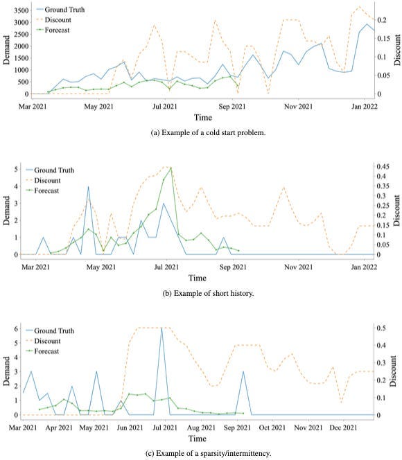
The major contributions/key points of this paper are:
- Covariate Handling: Using discount as a dynamic covariate.
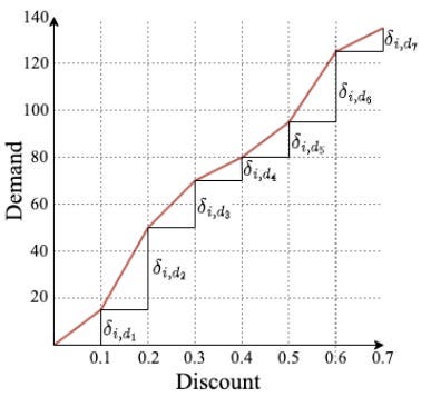
- Causal Relationship: Enforcing a monotonic relationship between discount and demand via a piecewise linear function parameterized by feedforward networks.
- Two forecasting modes: Training and predicting short- and long-term demand with a single global model.
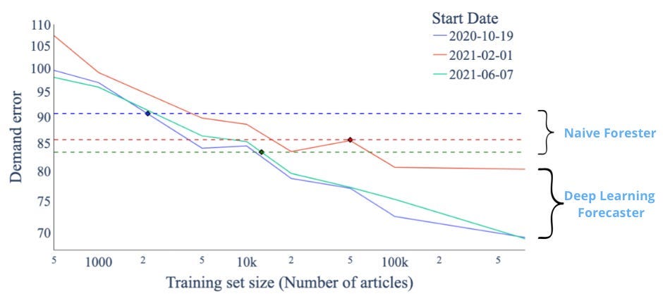
- Scaling laws: Demonstrating the first sparks of scaling laws in Transformer forecasting models.
First, the authors explain how they configured the forecasting problem by translating the sales observations into demand forecasting. Demand planning is the most common case in retail forecasting.
Also, the authors cleverly impute demand (e.g., it can happen when there’s a stock shortage) instead of marking it as missing.
Note: Demand Forecasting is the first and most important step in a supply forecasting pipeline
Demand represents what customers want to buy, while sales are restricted by stock availability. Forecasting demand is crucial, as it reflects true customer needs, unlike sales, which are supply-dependent.
If sales drop to zero due to stock shortages, future forecasts based on sales will also reflect zero. This can mislead automated supply planning systems, leading to no new orders.
To ensure an efficient supply chain, always forecast demand instead of sales. Accurate demand forecasts prevent disruptions and maintain stock to meet customer needs.
Zalando’s Forecasting Pipeline
The paper categorizes features into 4 types:
- static-global: time-independent & market-independent
- dynamic-global: time-dependent & market-independent
- dynamic-international: time-dependent & market-specific
- static-international: time-independent & market-specific

While all covariates enhance performance, discount is the most influential. Also, data has a weekly frequency.
The Zalando team trained a global Transformer model with:
- Input: A single tensor of dimension R𝑡×𝑢×𝑣, where 𝑡 is the time dimension, 𝑢 the batch size and 𝑣 the dimension of the covariate vector.
- Output: near future is 5 weeks and far future is 5 to 20 weeks.
The authors input details for different products, markets, and discount levels — and the output of the forecasting engine is a 𝑅𝑎×𝑐×𝑡×𝑑 tensor that spans over 𝑡 = 26 future weeks, up to 𝑎 = 1 × 10⁶ products, 𝑐 = 14 countries and 𝑑 = 15 discount levels.
Figure 2 describes the top-level view of the Transformer model:
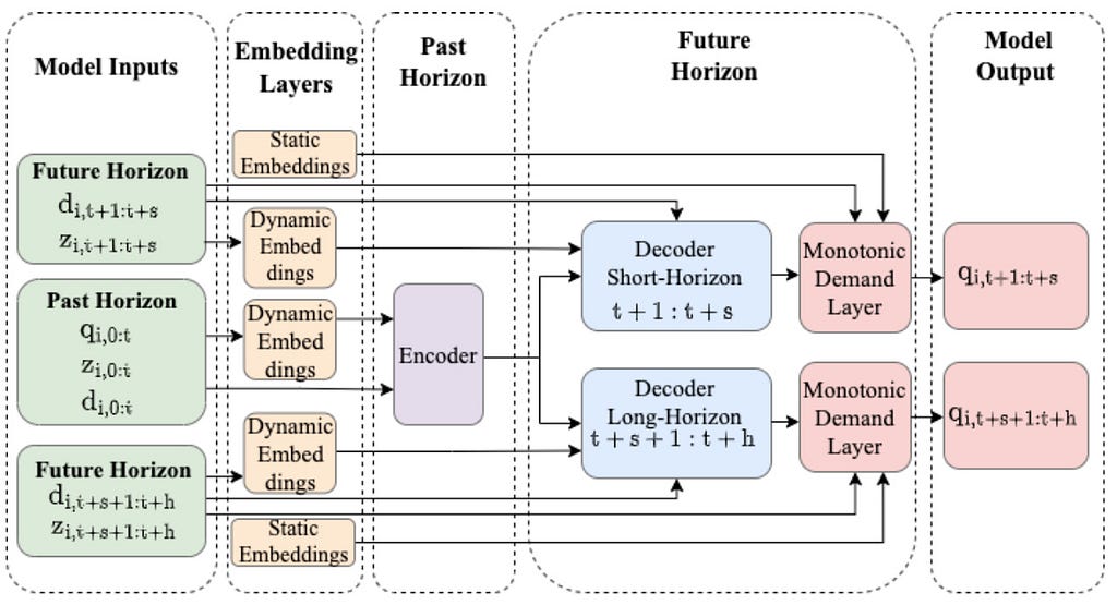
The model uses an encoder-decoder structure with time-series-specific adaptations:
- Encoder: Processes past observed covariates.
- Decoder: Handles future known inputs, generating short and long-term forecasts.
- Non-autoregressive Decoder: Produces forecasts in a multi-step manner.
- Positional Embeddings: They are not added to tokens as in the traditional Transformer — but as an extra covariate.
The key innovation was natively embedding the idea of a monotonic increase in demand with higher discounts into the model.
This makes sense since the 2 values are positively correlated — but if this relationship is not imposed in the model, it won’t necessarily occur all the time.
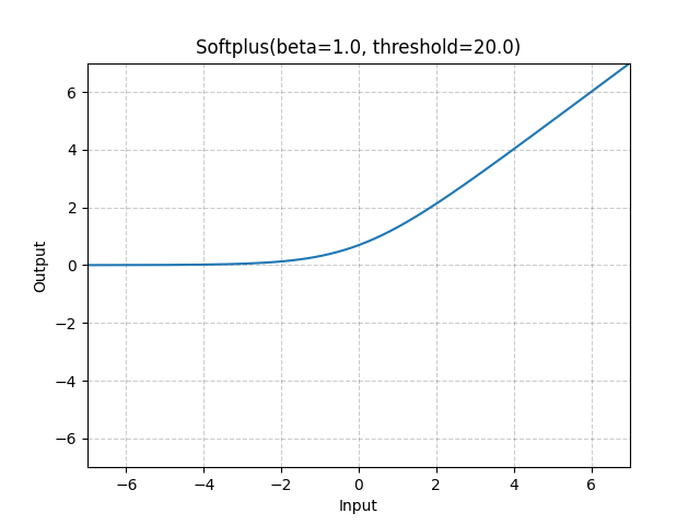
Future demand for a given discount is modeled via a piecewise linear, monotonic demand response function. This function is parameterized by 2 FFNs in the Monotonic Demand Layer. A softplus transformation ensures the demand function is monotonically increasing w.r.t. to discount:
Finally, an important aspect of this paper was the first spark of scaling laws in forecasting. It was the first time a paper showed on a private, large, and diverse dataset that a Transformer-based forecasting model leveraged scale to deliver better performance:
This work established a foundation for large-scale, time-series forecasting models.
In general, it’s a well-written paper with interesting details that we didn’t cover here — but we’ll discuss them in a future article. Stay tuned!
Forecasting Reconciliation: A Review
Hierarchical forecasting and reconciliation are among the most active areas in time-series research.
It all started with a research team at Monash University (which included the distinguished professor Rob Hyndman) publishing the iconic paper [Hyndman et al., 2011]. Of course, work on this area had started earlier.
Hierarchical forecasting reached the broader machine-learning community through the M5 forecasting competition.
The paper [2] written by the same school of thought researchers is the best resource for tracking the latest forecasting reconciliation research.
Preliminaries on Forecasting Reconciliation
Consider a hierarchical time series with multiple levels, such as product and store. Your task is to forecast for all levels.
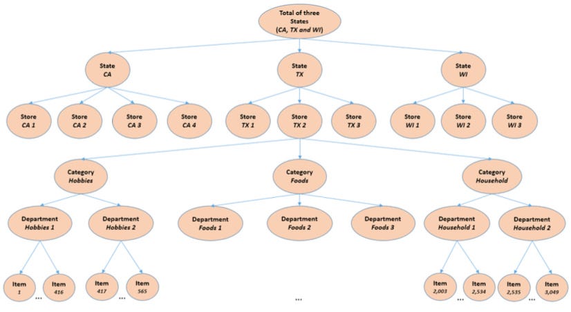
- Naive approach: We separately forecast sales for each product, store, and the total. However, the top-level forecasts won’t align with the sum of the lower levels, making them incoherent.
- Bottom-up approach: Here, forecasts start at the bottom level and aggregate upwards. This avoids information loss but isn’t optimal. Lower-level series are often noisy or sparse, causing errors to accumulate as you aggregate.
Other approaches, like top-down and middle-out, have similar challenges.
The best way is to establish a mathematical reconciliation method:
Forecasting reconciliation is not a time-series model, but a process that ensures consistency across different levels of forecasts. Given base forecasts across all levels, this process optimally makes base forecasts coherent.
✅ Note: Some models generate coherent forecasts directly (see [2]).
Why Use Forecasting Reconciliation?
Tutorials often present forecasting reconciliation as a way to ensure forecasts make sense, avoiding questions from a manager like why the sum of product A and B sales doesn’t match the total estimate.
Ok, this is also true. But that’s not all.
Reconciliation often improves forecast accuracy in hierarchical datasets. Here’s why:
- You can use the best model for each level.
- For example, models at different levels can leverage distinct loss functions (e.g., Tweedie loss for non-negative, right-skewed lower-level data; Huber loss at the top levels for outlier-prone top levels).
Once you’ve generated the base optimal forecasts at each level, you can select an appropriate reconciliation method from [2]. And just like that — boom! Your forecasts will not only be coherent but also likely more accurate overall!
Some Notation
Let’s break down hierarchical forecasting.
Suppose we have 3 stores, each selling 2 products. This setup gives us 10 time series in total, with 6 at the bottom level.
For instance, yA,t represents the sales of store A at time t and yAA,t represents the sales of product A. The top-level yt aggregates total sales.
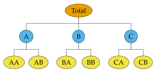
The equations which describe this graph are the following:

The equations describing this hierarchy are as follows:
The vector yt represents the total sales, S is the matrix summing these observations, and bt is the vector of bottom-level observations/sales at time t.
Let’s zoom into the values of the above equation:
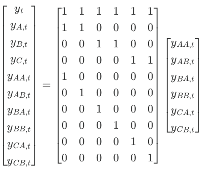
Hence, the summing matrix S determines the hierarchical structure.
Bottom-Up Approach
Reconciliation aims to adjust incoherent base forecasts to make them coherent and as accurate as possible.
We achieve this using a projection (or reconciliation) matrix G:
where:
- y_tilde: reconciled forecasts at all levels
- S: summing matrix
- G: projection matrix
- yhat: base forecasts at all levels
- h: horizon
and in matrix format:
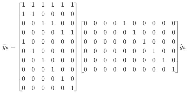
Notice that in G, the first 4 columns zero out the base forecasts at the bottom level, and the other columns pick only the base forecasts of the bottom level.
Advanced Reconciliation Methods
The bottom-up approach is straightforward — it aggregates forecasts to ensure coherence.
However, it’s not a native reconciliation method since forecasts are made coherent simply by aggregation.
That’s why the bottom-up approach has a simple projection matrix G, but in practice, we can devise a reconciliation method by solving for the matrix G.
The goal is to find the optimal G matrix according to equation 6 that gives the most accurate reconciled forecasts.
The paper starts with the simple OLS equation for estimating G:
G = (S'S)^-1 S'
And continues with the milestone paper Wickramasuriya et al. (2019) which introduces the MinTrace (MinT) method that minimizes the sum of variances of the reconciled forecast errors.
The matrix G is then computed as:
G = (S'W^(-1) S)^-1 S' W^(-1)
where Wh is the variance-covariance matrix of base forecast errors.
We won’t go into further details here, feel free to read the original paper[2].
Key Challenges and Tools
The authors discuss additional reconciliation approaches and how these can be enhanced with probabilistic forecasting or accelerated using sparse methods. However, reconciliation methods can be memory-intensive, especially with datasets containing hundreds of time series.
They also cover domain-specific applications of hierarchical forecasting and review software tools and libraries for implementation.
The paper is detailed and well-written but assumes some familiarity with the field. For beginners, I recommend Rob Hyndman’s and George Athanasopoulos’s Forecasting: Principles and Practice book which has a chapter dedicated to hierarchical forecasting.
TSMixer: An All-MLP Architecture for Time Series Forecasting
Boosted Trees excels at forecasting tabular-like time series data with multiple covariates.
However, deep learning models have struggled to leverage their architectures effectively on complex datasets due to overfitting issues.
Google researchers addressed this by developing TSMixer, a lightweight MLP-based model, and its enhanced variant, TSMixer-Ext, which accommodates exogenous and future-known variables. TSMixer-Ext delivered a remarkable performance in Walmart’s M5 competition, surpassing established SOTA models.
TSMixer stands out for its double-mixing operation, utilizing cross-variate information across both the time domain (time-mixing layer) and feature domain (feature-mixing layer).
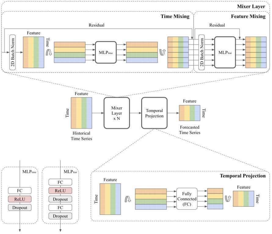
We covered TSMixer and TSMixer-Ext in detail in the article here — check it out for more insights!
Find a hands-on tutorial on TSMixer in the AI Projects folder (Project 8)
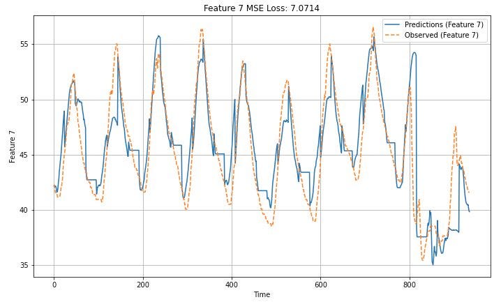
CARD: Channel Aligned Robust Blend Transformer for Time Series Forecasting (ICLR 2024)
The release of the DLinear and TSMixer papers exposed weaknesses in Transformer-based forecasting models.
In multivariate setups (where models learn cross-variate dependencies across all time series and predict them jointly), Transformers often overfit.
The quadratic self-attention mechanism tended to capture noise, limiting performance — especially on smaller or toy datasets. As a result, newer attention-based approaches shifted to univariate training, yielding impressive results.
CARD revisits the multivariate scenario, aiming for SOTA results by redesigning attention mechanisms for time series.
Dual Channel Attention
Earlier, we saw how TSMixer uses a double MLP mixing operation across time and feature dimensions. Similarly, CARD applies attention across both token (time) and channel (feature) dimensions:
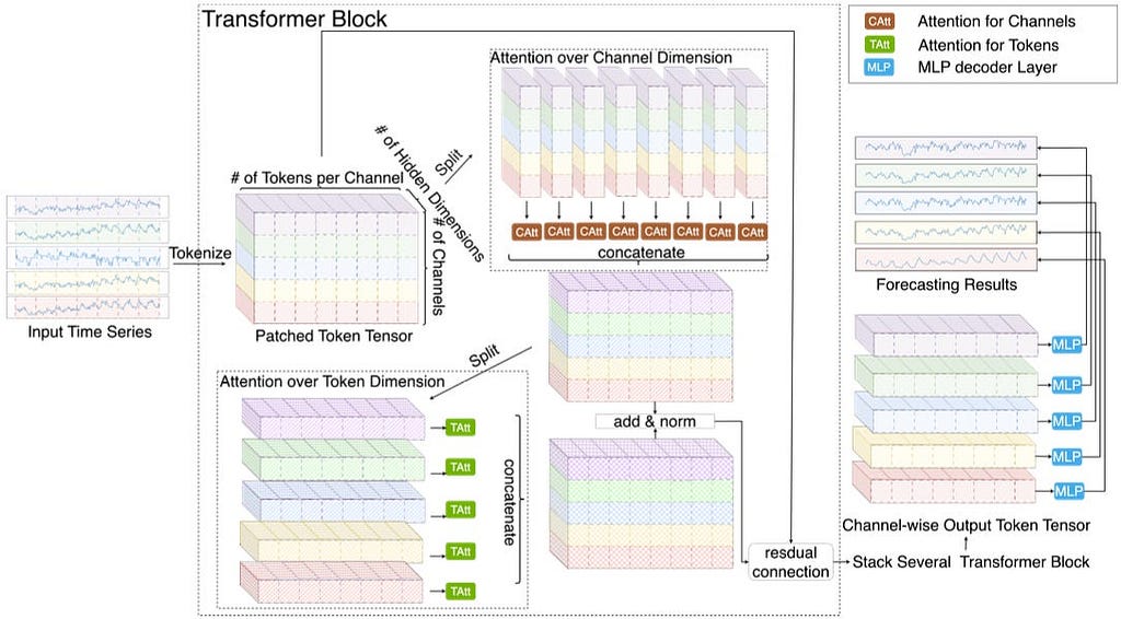
Figure 10 is very similar to TSMixer’s architecture in Figure 8. The authors sparsify attention further with summary tokens, exponential smoothing, and extra projections. These additions reduce complexity (Figure 11), helping the model distill meaningful information.
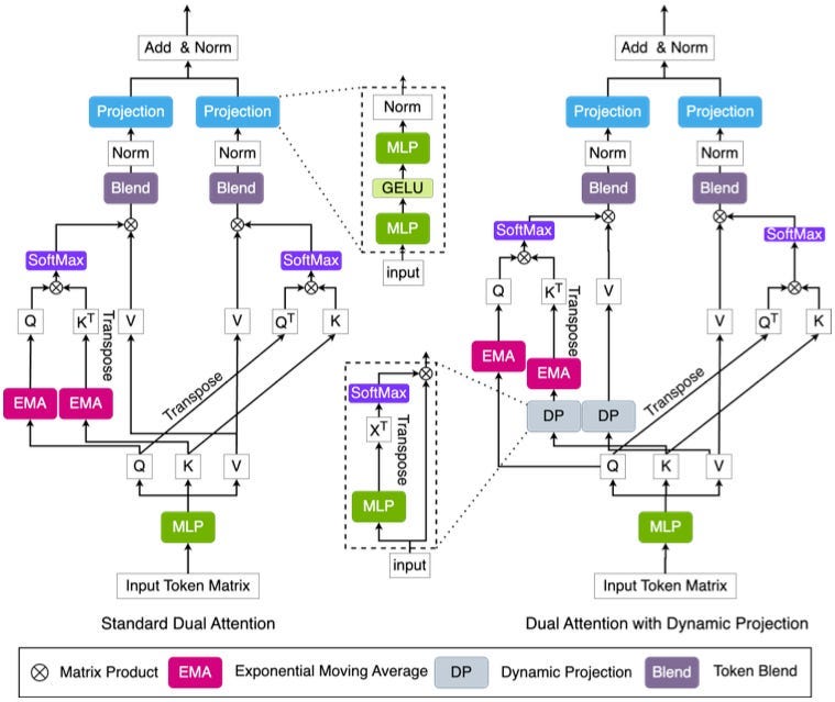
Note: CARD partitions signals into patches, meaning tokenization occurs at the patch level.
Patching benefits attention-based models because point-wise tokenization lacks semantic richness, while patches better capture a sequence’s characteristics.
Token Blend Module
In Transformer forecasting, each attention head focuses on specific aspects of the data or feature patterns in the input sequence. For example:
- One head might focus on short-term dependencies (e.g., relationships between nearby time steps).
- Another might capture periodic behavior (e.g., weekly or seasonal cycles).
Thus, within a single attention head:
- Tokens encode related information about the input sequence, filtered through the head’s particular “lens” or learned feature pattern.
- Tokens adjacent to each other correspond to neighboring time steps in the sequence and share temporal proximity.
In vanilla attention, tokens merge across heads. The proposed token blend module(Figure 12) modifies this by merging adjacent tokens within the same head after multi-head attention, creating tokens for the next stage:

Since each attention head specializes in specific features (e.g., trends or periodic patterns), merging tokens within the same head retains this focus while expanding the temporal scope.
Signal Decay-Based Loss Function
The authors note that errors are higher at the far future end of the horizon. Near-future predictions contribute more to generalization improvements than far-future ones.
To address this, they use a decay-based loss function — a MAE-based variant that weights near-future predictions more:
where:
- a_t(A) are the observations at time t, given historical information A
- ahat_t are the predictions at time t, given historical information A
- L is the sequence length
Hence, this loss emphasizes near-future accuracy more.
In general, CARD is an impressive model. Unfortunately, it hasn’t been integrated into any known forecasting library, but the authors have open-sourced it. I’ll definitely create a tutorial on this model in future articles.
Spacetimeformer
The paper “Long-Range Transformers for Dynamic Spatiotemporal Forecasting[5]“, introduced a new model called Spacetimeformer.
What makes Spacetimeformer advantageous?
There are 3 key levels in general:
- Temporal Models: Traditional attention-based time series models represent multiple variables per timestep in a single token, overlooking spatial relationships between features (Figure 13b).
- Graph Models: Graph attention models manually encode feature relationships using static, hardcoded graphs, which cannot adapt over time (Figure 13c).
- Spatiotemporal Models: Spacetimeformer integrates temporal and spatial attention, representing each feature’s value at a specific timestep as an individual token. This approach captures complex interactions across space, time, and value (Figure 13d).
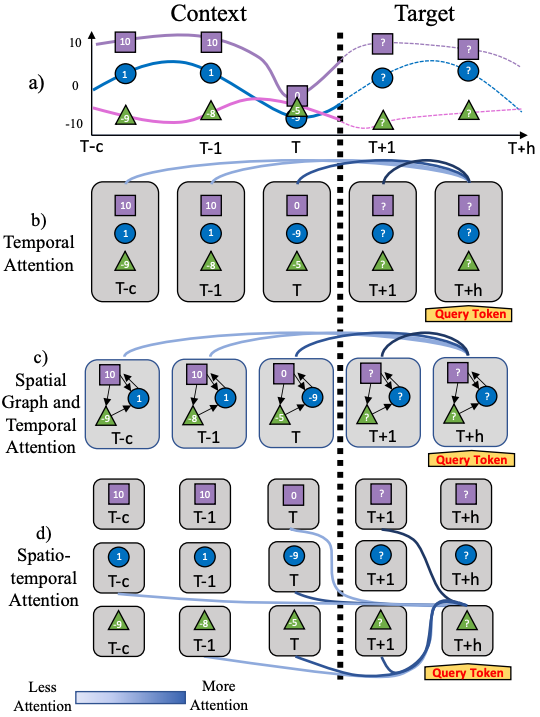
Previous Transformer-based models used one input token per timestep so that the embedding of the token at time 𝑡 represents 𝑁 distinct variables at that moment in time.
This is problematic because:
- Lagged Information: In practice, dependencies can be lagged, such as y depending on xi-1 rather than xi. Time-based embeddings may overlook these lags.
- Limited Receptive Field: Unlike NLP, where vocabularies are discrete, time-series data are continuous. Tokenizing by timepoints restricts receptive fields, limiting the capture of long-term, cross-temporal correlations.
Spacetimeformer’s Solution
Spacetimeformer addresses these limitations with the architecture shown in Figure 1d. For 𝑁 variables and a sequence length of 𝐿, we have:
Multivariate inputs of shape (𝐿, 𝑁) are flattened into sequences of shape (𝐿 × 𝑁, 1), where each token represents a single variable’s value at a specific timestep. This transformation enables the model to jointly learn attention across both space and time, creating the “spatiotemporal attention” mechanism illustrated in Figure 13D:
The embedding differences between a temporal and a SpatioTemporal model are shown in Figure 14:
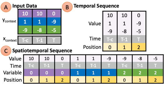
Figure 14 shows in detail the embedding types used by SpaceTimeFormer:
- Given Embeddings: Multivariate inputs include time information, with missing values (“?”) set to zero for predictions. These embeddings indicate whether values are provided as context or require prediction
- Time Embeddings: Time sequences are passed through a Time2Vec layer to create time embeddings that capture periodic patterns.
- Variable Embeddings: Each time series covariate is mapped to a spatial representation using a lookup-table embedding.
- Value & Time Embeddings: Time2Vec embeddings and variable values are projected using a feed-forward layer.
- Position Embeddings: Typical learned position embeddings used in other models like BERT (not shown in Figure 15)
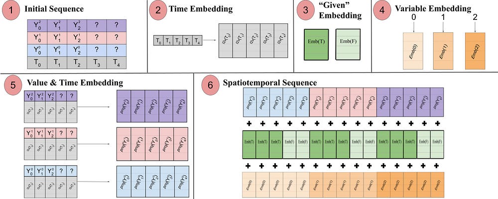
All embeddings are summed to model relationships across temporal and variable spaces, but this increases input sequence length.
Given self-attention’s quadratic complexity, scaling becomes challenging for large N values. To address this, the following optimizations are applied:
- Performer’s FAVOR+ Attention: A linear approximation of attention using a random kernel method.
- Global and Local Attention: Local attention allows each token to focus on its spatial variable’s timesteps, while global attention lets tokens attend across the entire spatiotemporal sequence. This reduces computations without compromising temporal dynamics.
Figure 16 illustrates SpaceTimeFormer’s encoder-decoder architecture:
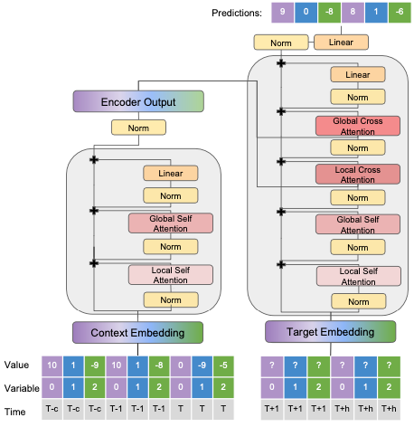
Benchmark results show promising performance, with the model outperforming other notable implementations. Newer models like the ITransformer and CARD we saw earlier have since adopted the embedding mechanism across the time dimension.
Finally, attention weights can be extracted and visualized to reveal spatiotemporal relationships among variables:
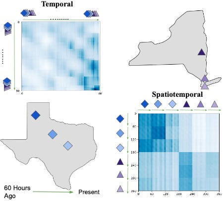
You can find the official repo of SpaceTimeReformer here. This model has also been applied for other cases such as financial forecasting.
References
[1] Kunz et al. Deep Learning based Forecasting: A case study from the online fashion industry
[2] Athanasopoulos et al. Forecast reconciliation: A review
[3] Chen et al. TSMixer: An All-MLP Architecture for Time Series Forecasting
[4] Xue et al. CARD: Channel Aligned Robust Blend TransFormer For Time Series Forecasting (ICRL 2024)
[5] Grigsby et al. Long-Range Transformers for Dynamic Spatiotemporal Forecasting
Thank you for reading!
Influential Time-Series Forecasting Papers of 2023–2024: Part 1 was originally published in Towards Data Science on Medium, where people are continuing the conversation by highlighting and responding to this story.
from Datascience in Towards Data Science on Medium https://ift.tt/JirWqON
via IFTTT


