Predicting a Ball Trajectory
Polynomial Fit in Python with NumPy

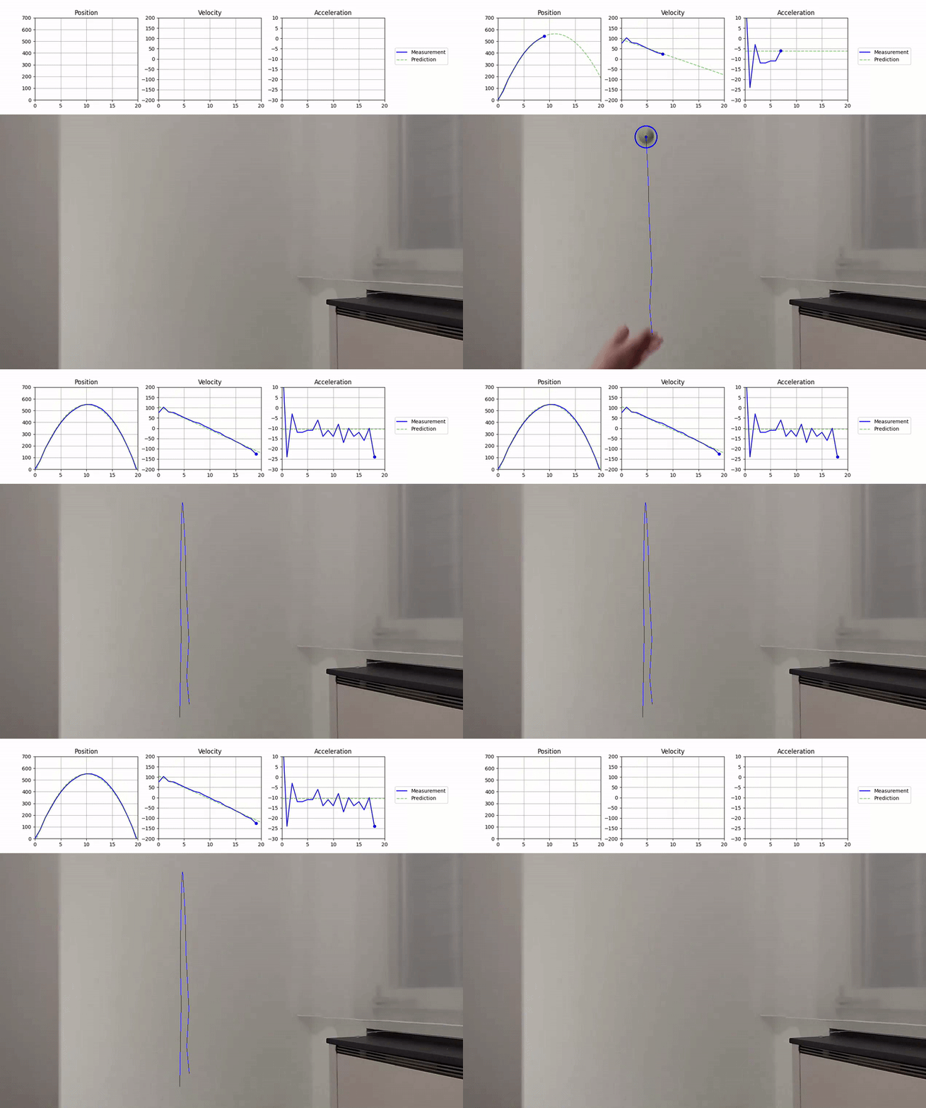
In a previous project I visualized the trajectory of a ball that I threw vertically into the air with a real-time position, velocity and acceleration plot. Extending upon this project, I wanted to calculate and visualize a trajectory prediction based on a simple physics model. In this post, I will explain how I fit the model to the measured state of the ball and visualize the predicted trajectory.

Physics Model
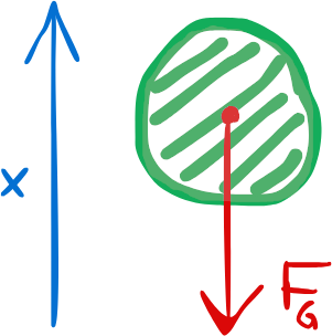
Let’s start with the physics model for the ball. For simplicity, I am only considering the vertical movement of the ball, simplifying the problem to a one-dimensional one. Furthermore, I am only modelling the ball as soon as it leaves my hand and neglecting any air drag. This simply leaves us with a single constant force acting on the ball: gravity.

The force is calculated with the mass of the ball and the gravitational acceleration g, which is approximately 9.8m/s², depending on location and altitude. The change in altitude of the ball is so small that the change in g is negligible and we can assume it to be constant. Notice that I define the position axis pointing upwards, opposite to the gravity vector, resulting in a negative sign for the force.

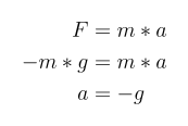
Based on Newton’s second law, we can derive the acceleration of the ball to be equal to the gravitational acceleration, as the mass cancels out during calculation.

Since acceleration is the time derivative of velocity, and velocity itself is the time derivative of the position, we can derive the motion equations by integration. Assuming the acceleration is constant, we get the following equations for the velocity and position:

In summary our physics model results in a constant acceleration, linear velocity and quadratic position. Or in other terms, all three functions are polynomials of different degrees:
- Acceleration is constant, a polynomial of degree 0
- Velocity is linear, a polynomial of degree 1
- Position is quadratic, a polynomial of degree 2
We will use this information in the next chapter to find the best fit for the parameters of the functions.
Polynomial Fit
Now on to the coding part, where we translate this into Python code. Our starting point is the code from the previous project, where we have three numpy arrays containing our extracted position and approximations of the velocity and acceleration values:
pos = np.array([tracked_pos[0][1] - pos[1] for pos in tracked_pos])
vel = np.diff(pos)
acc = np.diff(vel)
To fit our polynomials, we can use the numpy function polyfit. The function takes in two arrays and a degree of the polynomial. The first input array is the time-axis and the second array is the value at each timestamp. In our case we can define the time steps as follows:
t_pos = np.arange(len(pos))
t_vel = np.arange(len(vel))
t_acc = np.arange(len(acc))
NOTE: Since we use an approximation based on the array differences for the velocity and acceleration, they all have different lengths and we need to define a time axis for each function separately.
Now we can pass the time-axis and the arrays to the polyfit function with the respective polynomial degrees.
poly_pos = np.polyfit(t_pos, pos, deg=2)
poly_vel = np.polyfit(t_vel, vel, deg=1)
poly_acc = np.polyfit(t_acc, acc, deg=0)
The resulting arrays will contain the parameters for the polynomials of the respective degree with the highest order coefficient first.
Visualize Predictions
To show the fitted polynomial functions, we need to evaluate and plot the polynomial at each time step. I always want to show the polynomial predictions for the full time frame of the video sequence and a couple frames into the future.
t_pred = np.arange(num_frames + 5)
Now we can use the polyval function to evaluate the polynomials at each of the time step.
polyval_pos = np.polyval(poly_pos, t_pred)
polyval_vel = np.polyval(poly_vel, t_pred)
polyval_acc = np.polyval(poly_acc, t_pred)
Now you can simply show the static plots of these polynomial functions with matplotlib after the video ends. This will show the final prediction, the best fit based on all data points of the video.
fig, axs = plt.subplots(nrows=1, ncols=3, figsize=(12, 3), dpi=100)

axs[0].set_title("Position")
axs[0].set_ylim(0, 700)
axs[1].set_title("Velocity")
axs[1].set_ylim(-200, 200)
axs[2].set_title("Acceleration")
axs[2].set_ylim(-30, 10)

for ax in axs:
    ax.set_xlim(0, num_frames)
    ax.grid(True)

axs[0].plot(t_pred, polyval_pos, c="g", linestyle="--", alpha=0.5)
axs[1].plot(t_pred, polyval_vel, c="g", linestyle="--", alpha=0.5)
axs[2].plot(t_pred, polyval_acc, c="g", linestyle="--", alpha=0.5)

plt.show()
For some styling of the plots I used a semi-transparent green dashed line.

Animate Predictions
Similar to the last post, we can also show the prediction in real-time while the video is running. To make this as efficient as possible, I will again use the blit technique to not re-draw the full plot every frame.
To use this technique, we first have to create a reference of the lines object in the figure before the video loop with empty arrays. I also added a label for these lines to create a legend later on.
pl_pos_pred = axs[0].plot(
    [], [], c="g", linestyle="--", label="Prediction", alpha=0.5
)[0]
pl_vel_pred = axs[1].plot(
    [], [], c="g", linestyle="--", label="Prediction", alpha=0.5
)[0]
pl_acc_pred = axs[2].plot(
    [], [], c="g", linestyle="--", label="Prediction", alpha=0.5
)[0]
I also added the label to the plots of the measurements:
pl_pos = axs[0].plot([], [], c="b", label="Measurement")[0]
pl_vel = axs[1].plot([], [], c="b", label="Measurement")[0]
pl_acc = axs[2].plot([], [], c="b", label="Measurement")[0]
NOTE: The plot function returns a list of lines. Since we only create one line for each of our subplot plot function calls, we need to reference the first element in this list, hence the array indexing [0] at the end of these lines.
Now instead of plotting the predictions at the end of the loop, we can update the line plots in the loop the same way we updated the tracking plots in the initial post.
# Update Tracking Plots
pl_pos.set_data(t_pos, pos)
pl_vel.set_data(t_vel, vel)
pl_acc.set_data(t_acc, acc)

# Update Prediction Plots
pl_pos_pred.set_data(t_pred, polyval_pos)
pl_vel_pred.set_data(t_pred, polyval_vel)
pl_acc_pred.set_data(t_pred, polyval_acc)
One thing we need to be careful of now that we update the predictions every step of the loop, is that we don’t try to predict before we have any data points, as this will raise an exception in the polyfit function. To prevent this, we can simply check that all our tracking variables contain values.
if len(pos) > 0 and len(vel) > 0 and len(acc) > 0:
    poly_pos = np.polyfit(t_pos, pos, deg=2)
    poly_vel = np.polyfit(t_vel, vel, deg=1)
    poly_acc = np.polyfit(t_acc, acc, deg=0)

    ...
Next we need to re-draw these lines for each plot axis by restoring the background and calling the draw_artist function for each line.
# Position
fig.canvas.restore_region(bg_axs[0])
axs[0].draw_artist(pl_pos)
axs[0].draw_artist(pl_pos_pred)
axs[0].draw_artist(mark_pos)
fig.canvas.blit(axs[0].bbox)

# Velocity
fig.canvas.restore_region(bg_axs[1])
axs[1].draw_artist(pl_vel)
axs[1].draw_artist(pl_vel_pred)
axs[1].draw_artist(mark_vel)
fig.canvas.blit(axs[1].bbox)

# Acceleration
fig.canvas.restore_region(bg_axs[2])
axs[2].draw_artist(pl_acc)
axs[2].draw_artist(pl_acc_pred)
axs[2].draw_artist(mark_acc)
fig.canvas.blit(axs[2].bbox)
For the final touch, I added the legend to the right side of the figure. To make sure that it fits, we can adjust the subplots slightly to the left.
# make space for the legend
fig.subplots_adjust(left=0.05, bottom=0.1, right=0.85, top=0.85)

# show legend in the right center of the figure
handles, labels = ax.get_legend_handles_labels()
fig.legend(handles, labels, loc="right")
And here you go, the optimized, animated plot of the tracked trajectory. Check out the full source code for some more details, such as the marker on the current state of the ball.

Conclusion
In this project, you learned how to use a simple physics model and polynomial fitting to predict the trajectory of a ball in motion. We used blitting to visualize the trajectory plots in real-time and overlay the predictions on top of the measured state of the ball.
If you want to learn in detail how I created the animated plots and extracted the position, velocity and acceleration from the video, check out my first article:
Dynamic Visualizations in Python
The full source code is available from my GitHub below. If you have any questions don’t hesitate to ask, I am always happy to help. Take care!
All visualizations in this post were created by the author.
Predicting a Ball Trajectory was originally published in Towards Data Science on Medium, where people are continuing the conversation by highlighting and responding to this story.
from Datascience in Towards Data Science on Medium https://ift.tt/AapbdT3
via IFTTT


