Predictive Maintenance Models with a Focus on Class Balancing — Complete Notebook
Predictive Maintenance Models with a Focus on Class Balancing
From model creation to deployment: building a predictive maintenance system with streamlit
1. Overview
I am now going to take you through a project involving Predictive Maintenance Recommendation Systems integrated with IoT (Internet of Things) to reduce unplanned downtimes.
The idea is to utilize IoT sensor data from industrial equipment — of course, we’ll be working with fictitious data, but it will simulate what would be real data within a company.
We’ll use this data to create a fully machine-learning-based recommendation system. Along the way, I’ll place a strong emphasis on handling imbalanced data.
I’ll introduce at least 5 different techniques to you. We’ll create five model versions. In the end, we will select the best model, justify our choice, test the model, and then deploy it through a web application using Streamlit.
So, we have quite a bit of work ahead. The link to the project on my GitHub will be at the end of this tutorial, along with the bibliography and reference links for you to consult if you wish.
Let me know if this adjustment meets your expectations or if there’s anything else you’d like to modify!
Summary:
1. Overview
2. Installing and Loading Packages
3. Loading Data and Verifying Class Proportion
4. Data Preparation
5. Option 1: Model-Level Weight Adjustment (No Resampling)
6. Option 2: Undersampling the Majority Class
7. Option 3: Oversampling the Minority Class
8. Option 4: Automatic Balancing with SMOTE
9. Option 5: Automatic Balancing with SMOTE and LightGBM Algorithm
10. Model Selection — Which Model Would You Choose?
11. The Main Criterion for Model Selection
12. Testing the Model Deployment
13. Deploying the Model with Streamlit
14. Building the App
15. Project 13 — Conclusion
16. GitHub Project and Useful Links
2. Installing and Loading Packages
Let’s begin the execution of the project with the necessary Python packages for our work. We’ll head straight to the Notebook.
We start with the Watermark package to generate a watermark for the versions of the other packages.
# This package is used to record the versions of other packages used in this notebook.
!pip install -q -U watermark
After that, I will install two packages and then load some below.
Here’s a very important detail. Pay attention! I want to use a Python package that will help us perform class balancing:
!pip install -q imbalanced-learn==0.12.3
The package name is imbalanced-learn. However, there is a problem with this package. Initially, the package name was only imblearn.
The package exists and is listed on PyPI.

Look at the last time this package was updated: 2017. It’s been a long time. The package developers decided to change the name:

Use this name instead of using imblearn. The problem is that the imblearn package is still available and often even in some versions of Anaconda.

Then, if you use this name here, it will cause problems. This is because the package no longer has the necessary functions to perform the work.
The package to be used is imbalanced-learn. But now comes the part that really ties your brain in knots. Attention! Pay close attention! You install the package like this, but when you import it, you import it like this:
!pip install -q imbalanced-learn==0.12.3
But when you import, you only import it as imblearn:
from imblearn.over_sampling import SMOTE
That is, you will use the old package name when installing, but with the new name.
But when you import the package, you must only use imblearn. This can lead to a conflict.
Why? If the imblearn package is already installed locally, due to Anaconda Python, your code will try to use the old package, the outdated one.
It will not understand that it is supposed to use the new package. So, you must absolutely do the following:
pip uninstall imblearn
I do not recommend doing this through Jupyter Notebook. Because the pip uninstall, which uninstalls the package, will ask for confirmation.
So, it is possible that the notebook will freeze, continually prompting for confirmation and not executing.
Open a terminal, or command prompt, execute pip uninstall. Then you come back, clear the notebook, and execute again.
This is a typical package name conflict, which you can encounter with other Python packages as well. It's a free tool, provided by volunteers.
Resuming, let's then install the package in the appropriate version:
!pip install -q imbalanced-learn==0.12.3
The versions of the packages can be found at the end of the notebook.
I will primarily use the Random Forest algorithm. However, for one of the model versions, I want to introduce you to LightGBM.
This is a separate Python package, so you should install it in your environment as well:
!pip install -q lightgbm
After that, we import JobLib to save the models on disk.
We also use sklearn, which is scikit-learn with various algorithms for the project, along with NumPy and Pandas, the dynamic duo you're probably already familiar with:
# 1. Imports
import joblib
import sklearn
import numpy as np
import pandas as pd
import lightgbm as lgb
from sklearn.model_selection import train_test_split
from sklearn.ensemble import RandomForestClassifier
from sklearn.metrics import accuracy_score, roc_auc_score, classification_report
from sklearn.preprocessing import StandardScaler
from sklearn.utils import resample
from imblearn.over_sampling import SMOTE
The lightgbm, which I will use in one of the model versions, is designed specifically for machine learning tasks.
In sklearn, or scikit-learn, I utilize train_test_split to divide the data into training and testing sets.
The RandomForestClassifier algorithm and metrics such as accuracy_score, roc_auc_score, and classification_report are employed to compare the performance of different model versions.
For normalization, I’ll use StandardScaler. I will also work with resample, a technique for addressing imbalanced data, alongside SMOTE.
This latter technique is crucial for some of my strategies and is part of the imblearn package, which should be referred to as imbalanced-learn as noted in the pip install command.
Pay close attention to these details; they are subtle but make a significant difference. Now you can load the packages and activate the Watermark package, which displays the versions I am using. Let's proceed.
3. Loading Data and Verifying Class Proportion
We already have the Python packages; now we need the raw material — the data. Let’s proceed to load the CSV dataset:
# 2. Load the dataset
df = pd.read_csv('dataset.csv')
Let’s take a look at the shape:
# 3. Dataset Shape
df.shape

# -----> (10000, 6)
10,000 rows and 6 columns. Here, let me show you the head:
# 4. Dataset Sample
df.head()

So, observe that in the first few rows we have five predictor variables — input variables — and the output variable, maintenance_required.
As you know, to effectively work with machine learning, we need historical data. I require these IoT sensor readings, and for each reading, it’s crucial to determine whether the machine required maintenance or not.
We could have multiple readings for the same machine: perhaps one reading on one day and another the next day, or one hour and then the following hour. For each data reading, we must ascertain whether maintenance was necessary — yes or no. This requires someone to label the data accordingly.
Having just the IoT sensor data isn’t sufficient. It necessitates a labeling process based on historical data, which then enables us to attempt to predict the future. That’s precisely the essence of machine learning, right?
# 5. Dataset Information
df.info()
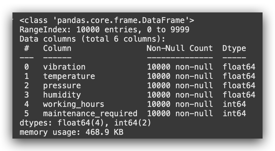
Here I have for you an info, a summary of the variable types. Our main focus here will be on addressing class imbalance.
So, we don't need to worry about missing values or anything like that at this point. Let's now check the class proportion:
# 6. Class Proportion
print(df['maintenance_required'].value_counts())
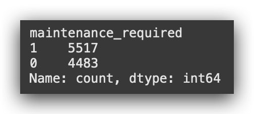
Class 1 is labeled ‘positive’ when maintenance is required, and Class 0, ‘negative’, when it’s not. These labels simply reflect whether a maintenance event occurred.
Such distinctions are crucial as they influence how a machine learning model interprets data, especially when one class is more prevalent.
This can skew the learning process, much like how focusing more on one subject over another can affect a student’s proficiency.
In practical terms, collecting more data from one class than another is common and typically not problematic. However, it does pose challenges during model training. Even a minor imbalance can be significant enough to necessitate corrective strategies.
I will address these challenges by introducing 5 different approaches aimed at balancing our data.
4. Data Preparation
Let’s now proceed with the data preparation, and then I will open up a very important discussion.
# 7. Separate explanatory variables (X) and target variable (y)
X = df.drop('maintenance_required', axis=1)
y = df['maintenance_required']
First, I will separate the variables into explanatory (X) and target (Y) sets.
In data science, these are also referred to as input variables, predictor variables, attributes, or features, depending on one’s professional background. However, they all mean the same thing.
Similarly, the target variable might be termed the output or dependent variable. There’s no uniform nomenclature for this either, but understanding the concept is what’s important.
For X, I will drop the maintenance_required variable; everything else becomes the input variable set.
The maintenance_required variable serves as my Y, the target variable, indicating whether maintenance was required—this is the outcome I am trying to predict using a machine learning model.
Next, we’ll divide the data into training and testing sets, maintaining an 80–20 ratio: 80% for training and 20% for testing.
This step is crucial for building effective machine learning models.
# 8. Split the data into training and testing sets (80% training, 20% testing)
X_train, X_test, y_train, y_test = train_test_split(
X, y, test_size=0.2, random_state=42)
Since this involves a random process, I’m using the random_state parameter to ensure you can reproduce the same results.
Class Balancing
With that set up, let’s open a discussion on why we apply class balancing only to training data.
From here, I will introduce a series of strategies, and I will consistently apply balancing to the training data, working exclusively with X_train.
The question is, why do we do this? There are several reasons:
1. Necessity for Training Only:
Class balancing is essential only for training the model. When using the test data, the model is already trained and ready.
The test data is merely for evaluating the model’s generalization ability. Therefore, applying class balancing to test data would be irrelevant and could skew evaluation metrics.
2. Avoiding Data Leakage:
During some unbalanced data treatment strategies, such as resampling, synthetic data is created.
If this resampling affected the entire dataset, synthetic data would end up in the test data, which is problematic.
Thus, strategies that modify data distribution should be applied solely to training data to prevent any data leakage. This separation ensures that the training process is the only phase affected by balancing.
3. Model Evaluation Integrity:
Implementing any balancing strategy on the entire dataset before splitting into training and test sets could influence the outcomes and performance metrics undesirably.
Unlike handling missing values, which must be addressed across the entire dataset to ensure consistency, class balancing is a methodological choice meant only to enhance training effectiveness.
4. Data Integrity:
Class balancing isn’t inherently a corrective action for a ‘problem’ in the data — it’s a strategy to make a model learn more effectively from an unrepresentative sample distribution.
Therefore, it’s crucial that this strategy does not interfere with the integrity of the test data, which should ideally reflect an unmanipulated real-world scenario.
Each strategy will be applied sequentially: I start with the first strategy and the initial division of X_train, then move on to the second, adjusting and evaluating each in turn. This methodical approach helps us identify the most effective strategy and ultimately choose the best model.
I will document these details in the notebook at the end of the tutorial, ensuring you have a full understanding of why and how we manage class balancing specifically within the training phase.
5. Model Weight Adjustment (No Resampling)
We can now explore Option 1, our initial strategy for managing imbalanced data.
This method involves adjusting the weights within the model, without resampling. By doing this, we address the class balance issue directly at the model level, meaning no alterations to the data itself are made.
From Option 2 onwards, I will reverse this approach. Instead of adjusting the model, I’ll focus on manipulating the data level.
This adjustment is crucial because not all models support direct weight modifications — Random Forest does, but others may not.
Let’s proceed to standardize the data to prepare for this strategy.
# 9. Standardize the data
scaler_v1 = StandardScaler()
X_train_scaled = scaler_v1.fit_transform(X_train)
X_test_scaled = scaler_v1.transform(X_test)
Attention: I will use X_train, and everything you do with the training data must also be applied to the testing data, right?
So, I'll create the standardizer scaler_v1. I'll apply fit_transform on the training data and transform only on the testing data. This way, the data is standardized.
Next, I’ll build the model using RandomForestClassifier. I'll configure it with 100 estimators and random_state=42 to ensure you can reproduce the same results.
And finally, here's a key detail, the secret to adjusting the model effectively:
# 10. Instantiate the model with class weight adjustment
model_v1 = RandomForestClassifier(
    n_estimators=100,
    random_state=42,
    class_weight='balanced'
)
I will set the class weight parameter to ‘balanced’. The default for this parameter is None.
So, if you don't specify anything, if you create the model like this:
# 10. Instantiate the model with class weight adjustment
model_v1 = RandomForestClassifier(
    n_estimators=100,
    random_state=42,
)
It will not concern itself with class balancing and will use the data as provided.
However, by setting this parameter, I am instructing the Random Forest, “You are receiving imbalanced data — assign different weights to each class.”
This means it will recognize the classes as having different weights, which they do, as we’ve seen due to their imbalance. This is the key to using this parameter.
By doing this, I do not need to manipulate the data myself; I let the model attempt to resolve this issue for us.
This method works well not only with Random Forest but also with XGBoost, another powerful ensemble method algorithm.
With other algorithms that do not offer this option, you would need to adjust the data directly.
This also brings us to the consideration of which algorithm to choose. If dealing with imbalanced data, an ensemble method is undoubtedly a good choice as it can handle this issue without requiring data manipulation.
Let’s now create model_v1 and proceed to the training phase:
# 11. Train the model and measure execution time
%%time
model_v1.fit(X_train_scaled, y_train)

Note that I am using the standardized training data, X_train_scaled, and the target variable, y_train.
It will take a few seconds, and the model will be successfully created.
Now, let’s proceed to make predictions:
# 12. Make predictions on the test set
y_pred = model_v1.predict(X_test_scaled)
y_pred_proba = model_v1.predict_proba(X_test_scaled)[:, 1]
I will first make predictions using the predict method, followed by predict_proba.
What’s the difference?
- predict: Provides the class prediction, either 0 or 1. The output is a binary classification result—one class or the other.
- predict_proba: Provides the probability for each class. Specifically, it returns two probabilities:
- The likelihood of the data belonging to class 0.
- The likelihood of the data belonging to class 1.
Why use both predictions?
- predict is used to calculate accuracy, as it provides the discrete class predictions.
- predict_proba is used to calculate the ROC AUC metric, as it requires the probabilities for both classes to generate the curve.
Different Metrics, Different Data
Each metric relies on distinct data types. To compute both accuracy and ROC AUC, I need to leverage both predict and predict_proba.
Test Data
Here, I use standardized test data, X_test_scaled, as input. This ensures the same scaling applied to training data is consistently used during testing.
With this input, the model generates predictions and probabilities for evaluation.
# 13. Model Evaluation
accuracy = accuracy_score(y_test, y_pred)
roc_auc = roc_auc_score(y_test, y_pred_proba)

print(f"\nAccuracy: {accuracy * 100:.2f}%")
print(f"AUC-ROC: {roc_auc * 100:.2f}%")
print("\nClassification Report:\n", classification_report(y_test, y_pred))
Now, I will compare the actual values with the predictions, calculate the metrics, and generate the classification report. Here’s the result:
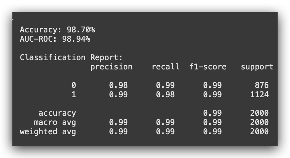
We achieved 98.7% accuracy, rounded to 99% AUC-ROC. Notice that all the metrics are very well-balanced, which is exactly what you want.
Accuracy is a global metric, while Precision, Recall, F1-score, and Support are local metrics. These are calculated separately for Class 0 and Class 1.
Ideally, these values should be close to each other — not identical, but similar enough.
If there’s a significant discrepancy between the metrics for the two classes, it is likely due to class imbalance.
This imbalance is something you typically want to avoid because it can cause the model to become skewed or less effective overall.
You aim for a model with a high capacity for generalization, and that’s what we achieved here. This is the first versionof the model, where we implemented a class balancing strategy at the model level.
Now, let’s save the model and the scaler to disk:
# 14. Save the model and scaler to disk
model_file = 'model_v1.pkl'
scaler_file = 'scaler_v1.pkl'

joblib.dump(model_v1, model_file)
joblib.dump(scaler_v1, scaler_file)

print(f"Model saved at {model_file}")
print(f"Scaler saved at {scaler_file}")

But did I apply the best strategy for class balancing? What’s your answer to that question? The answer is: I don’t know.That’s the honest response.
Do I have a way to determine if it’s the best strategy? No. To find out, what must I do? Compare it with another strategy.
Whenever you create only one model, you cannot definitively answer questions like: Is this the best model? Is this the best version? Was this the best strategy?
To answer these questions, I need to create at least one second version. Only then can I make a comparison.
6. Option 2: Undersampling the Majority Class
We applied the first strategy to address class imbalance. In Option 1, I didn’t modify the data and attempted to resolve the issue at the model level.
The performance is very good — excellent, in fact — but is this the best model?

Could I have applied the best strategy? To answer this question, I need to outline a different strategy, create another model version, and evaluate it.
This is how you determine whether a strategy is effective or not.
Let’s do this now with Option 2, where we apply undersampling of the majority class.
What does this mean? I will reduce the majority class, attempting to equalize it with the minority class. In other words, I will reduce the number of records for the majority class in our dataset.
I’ll demonstrate this process step by step. To make the concept even clearer, I’ll also include a cell showing the class proportion.
This will help you better understand the approach. Let’s start by bringing in the class proportion:
# 15. Class Proportion
df.maintenance_required.value_counts()
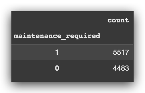
Observe: In Option 2, I will reduce the volume of data for Class 1. That’s the plan — undersampling.
But hold on. Does this mean you’ll reduce the total number of records for Class 1? So, you’ll reduce the size of the dataset? Yes, exactly that.
Will this have implications? Yes, it will. And this is precisely the point of discussion here. I want to show you the impact of each decision we make in this process.
To perform the undersampling, we’ll first concatenate the input and output data. This step is simply to make the process more manageable. Let’s proceed.
# 16. Concatenate X_train and y_train to facilitate resampling
train_data = pd.concat([X_train, y_train], axis=1)
Notice that I am working only with the training data, not the complete dataset.
First, we perform the concatenation. Then, we separate the majority and minority classes by filtering based on the class value, 1 or 0.
# 17. Separate the majority and minority classes from the training set
df_majority = train_data[train_data.maintenance_required == 1]
df_minority = train_data[train_data.maintenance_required == 0]
Remember, we apply sampling only to the training data.
Now, let’s check the size of both the majority and minority classes, specifically in the training set.
# 18. Check the size of the majority class
len(df_majority)

# -----> 4393

# 19. Check the size of the minority class
len(df_minority)

# -----> 3607
This confirms that the sizes are quite different from the totals in the complete dataset.

Now, let’s apply the undersampling. This is where I’ll use the resample function.
Where does it come from? It’s provided by Scikit-Learn, specifically in the utils module.
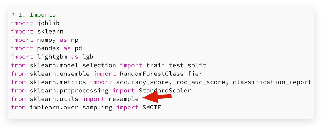
Let’s perform resampling, where I will reduce the majority class.
# 20. Apply undersampling to the majority class in the training set
df_majority_undersampled = resample(
    df_majority,
    replace=False,
    n_samples=len(df_minority),  # Match the size of the minority class
    random_state=42
Notice the parameters being used:
- replace=False: Ensures no duplication during resampling.
- n_samples: Matches the size of the minority class.
- random_state=42: Enables reproducibility of results.
After resampling, I’ll combine the undersampled majority class with the minority class.
# 21. Combine the minority class and the undersampled majority class
train_data_balanced = pd.concat([df_majority_undersampled, df_minority])
Now, I will prepare the input and output datasets again.
Why? Because earlier, in step #16, I combined them, right? I did that specifically to apply the resampling.
# 16. Concatenate X_train and y_train to facilitate resampling
train_data = pd.concat([X_train, y_train], axis=1)
So now, I need to separate the input and output data again. This step prepares the datasets for the next stage, which is training the model.
# 22. Split the balanced dataset into X_train and y_train
X_train_balanced = train_data_balanced.drop('maintenance_required', axis=1)
y_train_balanced = train_data_balanced['maintenance_required']
Let’s check the class balance in the training set:
# 23. Check the class balance in the training set
print(y_train_balanced.value_counts())
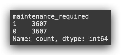
And there it is: 3,607 records, which matches the total for the minority class. This confirms that we’ve lost data. That’s the effect of the second strategy — undersampling. You lose records.
Now, imagine if I only had 100 records. Do you think it would make sense to apply undersampling? No. Why? Because you’d lose even more data. If you already have so few records, reducing them further isn’t feasible.
Undersampling is only a viable option when you have a large volume of data. Otherwise, you risk losing so many records that this strategy becomes counterproductive.
# 24. Standardize the data
scaler_v2 = StandardScaler()
X_train_scaled = scaler_v2.fit_transform(X_train_balanced)
X_test_scaled = scaler_v2.transform(X_test)
Now, we can proceed to standardize the data in step #24.
Why? Because earlier, I worked with the training data, and any transformations applied must ensure consistency for model training.
# 16. Concatenate X_train and y_train to facilitate resampling
train_data = pd.concat([X_train, y_train], axis=1)
Now that I’ve completed the resampling, I will proceed to standardize the data once again.
# 24. Standardize the data
scaler_v2 = StandardScaler()
X_train_scaled = scaler_v2.fit_transform(X_train_balanced)
X_test_scaled = scaler_v2.transform(X_test)
Notice that I’m now using scaler_v2. Next, I’ll create the model instance, naming it model_v2.
# 25. Instantiate and train the model
model_v2 = RandomForestClassifier(n_estimators=100, random_state=42)
Notice that now I’m no longer using the balanced parameter, which I applied in Option 1.
Why am I not using it here? Because this parameter only makes sense when the data is imbalanced.
Now that I’ve applied undersampling, the data is balanced, so there’s no need for it.

This parameter, which I used earlier, only makes sense if the data is imbalanced. Are the data imbalanced now? No.
I’ve just balanced them. Therefore, it doesn’t make sense to use the parameter in this case, right?
With this understanding, we can now proceed to create the model in step #25 and then apply the fit method to train it.
# 26. Train the model and measure execution time
%%time
model_v2.fit(X_train_scaled, y_train_balanced)

Training completed. Now, let’s proceed to make class predictions and probability predictions.
# 27. Evaluate the model on the test set
y_pred = model_v2.predict(X_test_scaled)
y_pred_proba = model_v2.predict_proba(X_test_scaled)[:, 1]
Next, we evaluate the model’s performance.
# 28. Model Evaluation
accuracy = accuracy_score(y_test, y_pred)
roc_auc = roc_auc_score(y_test, y_pred_proba)

print(f"\nAccuracy: {accuracy * 100:.2f}%")
print(f"AUC-ROC: {roc_auc * 100:.2f}%")
print("\nClassification Report:\n", classification_report(y_test, y_pred))

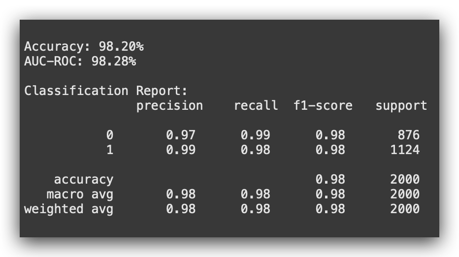
You may have noticed that the performance dropped slightly. Does this make sense? Yes, it does. Why? Because the volume of data decreased.
In other words, I provided fewer examples for the model to learn from. Naturally, with fewer examples, the model learned less.
This is evident in the slight decline of some metrics, such as precision. Despite this, the model in version 2 is still good. However, the drop in performance is clear, which is expected since we reduced the size of the dataset.
Now comes the next question: If you reduced the majority class, couldn’t you do the opposite? Couldn’t you increase the minority class instead?
Yes, you can, and that’s precisely what we’ll do in Option 3.
# 29. Save the model and scaler to disk
model_file = 'model_v2.pkl'
scaler_file = 'scaler_v2.pkl'

joblib.dump(model_v2, model_file)
joblib.dump(scaler_v2, scaler_file)

print(f"Model saved at {model_file}")
print(f"Scaler saved at {scaler_file}")

Let’s save model_v2 now, and then proceed to apply Option 3, which is the opposite approach—oversampling.
7. Option 3: Oversampling the Minority Class
We’ve applied undersampling, so now let’s try the opposite approach: oversampling. Instead of losing data, I’ll generate synthetic data.
In other words, I’ll use a resampling strategy to increase the size of the minority class.
You might be wondering: Wait a minute, are you creating synthetic data? Doesn’t that mean you’ll directly influence the dataset? Yes, that’s correct.
So, is there no perfect solution? No, there isn’t. It’s like the classic “short blanket” dilemma: if you cover your head, your feet are uncovered, and if you cover your feet, your head is exposed. That’s precisely the trade-off here.
At the end of the day, you need to experiment, compare versions, and decide what works best for each dataset and project. Let’s start again by concatenating the data.
# 30. Concatenate X_train and y_train to facilitate resampling
train_data = pd.concat([X_train, y_train], axis=1)
I’ll do this again because I’m returning to the original training data prepared at the beginning. This approach ensures that each strategy remains independent of the others.
So, I’ll concatenate the data once more and then separate the majority and minority classes.
# 31. Separate the majority and minority classes from the training set
df_majority = train_data[train_data.maintenance_required == 1]
df_minority = train_data[train_data.maintenance_required == 0]
The majority class is class 1, right?
And just a quick reminder: remember that resampling is applied only to the training data.
# 32. Check the size of the majority class
len(df_majority)

# -----> 4393


# 33. Check the size of the minority class
len(df_minority)

# -----> 3607
Just to reinforce this point, so there’s no confusion: what am I going to do now? I’m going to increase the minority class.
How do we do this? Once again, using resample.
# 34. Oversampling the minority class in the training set
df_minority_oversampled = resample(
    df_minority,
    replace=True,
    n_samples=len(df_majority),  # Match the size of the majority class
    random_state=42
)
The key difference lies in the number of samples. Now, I want the number of samples to match the length of df_majority.
To achieve this, I’ll set replace=True. What does this mean in practice? The minority class (df_minority) with 3,067 records will increase.
But how will it increase? Essentially, I’ll take existing data from the minority class, resample it, and create new synthetic data. This means the same data will be repeated, which is why replace=True is necessary.
If I used replace=False, what would happen? I would create a sample and discard existing data, which would result in insufficient records.
Therefore, replace=True ensures that some records will appear multiple times, allowing us to generate the required number of samples.
After this, we combine the majority and oversampled minority classes.
# 35. Combine the majority class and the oversampled minority class
train_data_balanced = pd.concat([df_majority, df_minority_oversampled])
I’ll now prepare X and y again.
# 36. Split the balanced dataset into X_train and y_train
X_train_balanced = train_data_balanced.drop('maintenance_required', axis=1)
y_train_balanced = train_data_balanced['maintenance_required']
Then, we check the class proportion.
# 37. Check the class balance in the training set
print(y_train_balanced.value_counts())
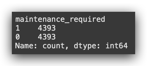
Look at what happened — it’s exactly the opposite of option 2, isn’t it? This time, I increased the minority class, effectively creating synthetic records based on the original data from the minority class.
In both option 2 and option 3, we had a direct impact on the data. As data scientists, we’re the ones making these changes.
But that’s the point: if no class balancing strategy is applied, the model can become imbalanced. That’s why applying at least one strategy is necessary to minimize this issue.
Notice that in options 2 and 3, we handled this manually. In option 4, I’ll soon demonstrate how to automate this process.
Now, let’s move forward and standardize the data.
# 38. Standardize the data
scaler_v3 = StandardScaler()
X_train_scaled = scaler_v3.fit_transform(X_train_balanced)
X_test_scaled = scaler_v3.transform(X_test)
I am creating the standardizer scaler_v3.
Next, we build the third version of the model.
# 39. Create the model
model_v3 = RandomForestClassifier(n_estimators=100, random_state=42)
We apply the fit method.
# 40. Train the model and measure execution time
%%time
model_v3.fit(X_train_scaled, y_train_balanced)

Wait a few moments to train the model.
Next, we make the predictions.
# 41. Evaluate the model on the test set
y_pred = model_v3.predict(X_test_scaled)
y_pred_proba = model_v3.predict_proba(X_test_scaled)[:, 1]
e, por fim, a avaliação do model_v3:
# 42. Model Evaluation
accuracy = accuracy_score(y_test, y_pred)
roc_auc = roc_auc_score(y_test, y_pred_proba)

print(f"\nAccuracy: {accuracy * 100:.2f}%")
print(f"AUC-ROC: {roc_auc * 100:.2f}%")
print("\nClassification Report:\n", classification_report(y_test, y_pred))

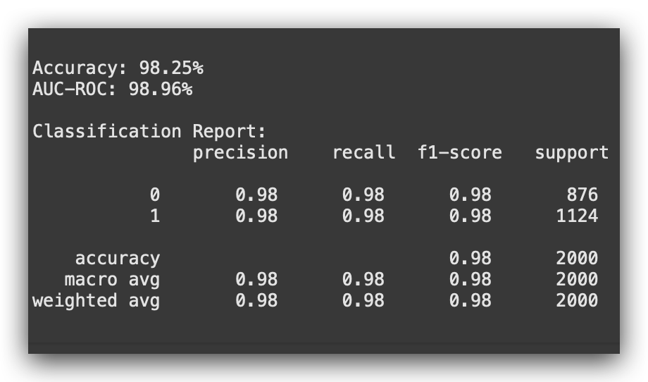
What do you observe? The accuracy improved slightly to 98.25%, compared to version 2. The AUC-ROC also increased slightly to 98.96%.
However, compared to version 1, which had an accuracy of 98.28%, the difference is minimal, right? This suggests that it might be worthwhile to focus on class balancing directly at the model level.
That said, keep in mind that not all models or machine learning algorithms offer a parameter like the one we used in option 1 with Random Forest.
Depending on the algorithm you choose, option 1 might not be available, forcing you to rely on versions 2 or 3 or other strategies we’ll explore later.
Finally, it’s worth emphasizing that all three models are good. The objective here is to identify the best version among them.
# 43. Save the model and scaler to disk
model_file = 'model_v3.pkl'
scaler_file = 'scaler_v3.pkl'

joblib.dump(model_v3, model_file)
joblib.dump(scaler_v3, scaler_file)

print(f"Model saved at {model_file}")
print(f"Scaler saved at {scaler_file}")

Let’s save version 3 to disk and proceed to version 4.
8. Option 4: Automated Balancing with SMOTE
We have already applied three strategies to handle class imbalance.
- Strategy 1 addressed the issue at the model level by leveraging a parameter provided by Random Forest. Not all algorithms offer such parameters.
- Strategies 2 and 3 involved manual adjustments at the data level. First, Undersampling reduced the majority class, followed by Oversampling, which increased the minority class.
Comparing performance, version 2 showed inferior results, explained by the reduction in data volume. Versions 1 and 3remain the most promising so far.
However, both version 2 and version 3 involved manual processes. In Option 4, we will automate class imbalance handling using SMOTE, an Oversampling technique.
SMOTE increases the minority class automatically and could potentially yield better results than manual methods.
Let’s begin. First, we’ll standardize the data.
You might wonder, “Why standardize now?” Don’t worry — I’ll explain shortly. For now, follow along with the sequence.
We start by standardizing the data:
# 44. Standardization
from sklearn.preprocessing import StandardScaler

scaler_v4 = StandardScaler()
X_train_scaled = scaler_v4.fit_transform(X_train)
X_test_scaled = scaler_v4.transform(X_test)
We now create the SMOTE instance:
# 45. Create the SMOTE instance
from imblearn.over_sampling import SMOTE

smote = SMOTE(random_state=42)
In practice, SMOTE is also an algorithm, isn’t it? It’s an algorithm that is pre-configured to generate synthetic data.
Here, we train the SMOTE algorithm using the standardized training data:
# 46. Train and apply SMOTE on the training set
X_train_smote, y_train_smote = smote.fit_resample(X_train_scaled, y_train)
So, I’ll create X_train_smote and y_train_smote. Why? Because we performed the resampling, which is Oversampling, but in an automated way.
Now, pay attention to this next step:
# 47. Check the size of the resampled training set
len(X_train_smote)

# -----> 8766
What is this number? 8786. On your machine, it might vary slightly, okay? In fact, all these results here could vary a bit depending on your hardware, due to the floating-point calculation precision of your processor.
Many people forget that all of this depends on the hardware where we run the software. The floating-point calculation precision of your processor can influence these results, but the general idea should remain more or less the same.
Why this number? 8786. That’s precisely what the algorithm did. In the case of SMOTE, it increased the minority class. As a result, it increased the data volume.
Previously, we defined the limit for this increase:

Exactly the length of df_majority. In the case of SMOTE, I didn’t set a specific limit. I let it generate synthetic data up to the amount it considers ideal.
In fact, this number, 8786, is based on the training process we performed with SMOTE. As such, it significantly increases the volume of data.
What impact does this have?
- The data volume increases considerably, leading to longer training times.
- Additionally, we are directly influencing the data.
In options 2 and 3, I manually influenced the data. Now, I’m doing so automatically using SMOTE.
Let’s proceed and create the model_v4:
# 48. Create the model
model_v4 = RandomForestClassifier(n_estimators=100, random_state=42)
After that, we trained the model:
# 49. Train the model and measure execution time
%%time
model_v4.fit(X_train_smote, y_train_smote)

The data volume isn’t excessively large, but it does take a bit more time. Let’s proceed to evaluate the model:
# 50. Evaluate the model on the test set
y_pred = model_v4.predict(X_test_scaled)
y_pred_proba = model_v4.predict_proba(X_test_scaled)[:, 1]
Let’s calculate the metrics and analyze the results:
# 51. Model Evaluation
accuracy = accuracy_score(y_test, y_pred)
roc_auc = roc_auc_score(y_test, y_pred_proba)

print(f"\nAccuracy: {accuracy * 100:.2f}%")
print(f"AUC-ROC: {roc_auc * 100:.2f}%")
print("\nClassification Report:\n", classification_report(y_test, y_pred))

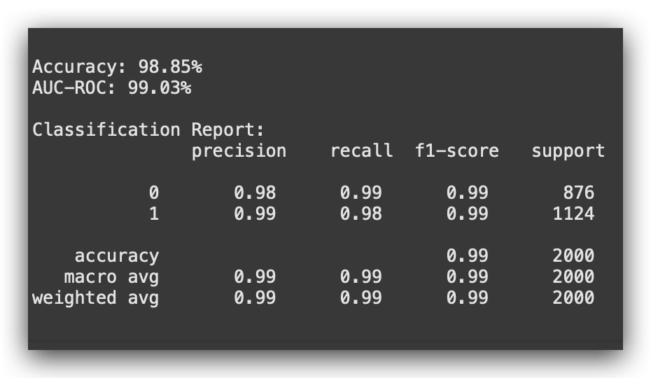
Version 4 improved both metrics — Accuracy and AUC-ROC — surpassing previous versions with SMOTE. Will this always happen? No.
Sometimes, SMOTE isn’t feasible due to data volume, limited control, or hardware constraints.
Options 2 and 3 are valid alternatives, while Option 1 avoids modifying data.
Option 4 fully automates class balancing, showing clear improvement. Remember, these metrics are based on test data — unseen during training.
Is this the best model version? So far, model_v4 is the strongest, but experimenting with modifications, like changing algorithms, might yield better results.
Let’s save version 4 and move to version 5:
# 52. Save the model and scaler to disk
model_file = 'model_v4.pkl'
scaler_file = 'scaler_v4.pkl'

joblib.dump(model_v4, model_file)
joblib.dump(scaler_v4, scaler_file)

print(f"Model saved at {model_file}")
print(f"Scaler saved at {scaler_file}")

For version 5, I’ll continue using SMOTE, as it delivered strong results.
However, I’ll switch the algorithm to evaluate whether Random Forest is influencing the performance in any way.
9. Option 5: Automatic Balancing with SMOTE and LightGBM Algorithm
In option 5, we’ll revisit the workflow between standardization and SMOTE, as the sequence directly impacts results.
In option 4, I intentionally standardized first, and now I’ll explain why.
Here, we’ll again use SMOTE for automatic balancing due to its strong results in option 4.
Additionally, I’ll replace Random Forest with LightGBM, allowing us to explore the new algorithm and evaluate if Random Forest affected performance positively or negatively.
Finally, I’ll demonstrate the order: applying SMOTE first, followed by standardization, to examine its impact.
%%time

# 53. Create the SMOTE instance
smote = SMOTE(random_state=42)

# 54. Train and apply SMOTE on the training set
X_train_smote, y_train_smote = smote.fit_resample(X_train, y_train)

# 55. Standardization
scaler_v5 = StandardScaler()
X_train_scaled = scaler_v5.fit_transform(X_train_smote)
X_test_scaled = scaler_v5.transform(X_test)

# 56. Create the model
model_v5 = lgb.LGBMClassifier(random_state=42)

# 57. Train the model with the SMOTE-balanced training set
model_v5.fit(X_train_scaled, y_train_smote)

# 58. Evaluate the model on the test set
y_pred = model_v5.predict(X_test_scaled)
y_pred_proba = model_v5.predict_proba(X_test_scaled)[:, 1]

# 59. Model evaluation
accuracy = accuracy_score(y_test, y_pred)
roc_auc = roc_auc_score(y_test, y_pred_proba)

print(f"\nAccuracy: {accuracy * 100:.2f}%")
print(f"AUC-ROC: {roc_auc * 100:.2f}%")
print("\nClassification Report:\n", classification_report(y_test, y_pred))
Next, I’ll reverse the order: standardizing first and applying SMOTE afterward. For simplicity, I’ve placed all the code in a single cell.
%%time

# 60. Standardize the variables
scaler_v5 = StandardScaler()
X_train_scaled = scaler_v5.fit_transform(X_train)
X_test_scaled = scaler_v5.transform(X_test)

# 61. Create the SMOTE instance
smote = SMOTE(random_state=42)

# 62. Apply SMOTE to the training set to handle class imbalance
X_train_smote, y_train_smote = smote.fit_resample(X_train_scaled, y_train)

# 63. Create the LightGBM model
model_v5 = lgb.LGBMClassifier(random_state=42)

# 64. Train the LightGBM model
model_v5.fit(X_train_smote, y_train_smote)

# 65. Evaluate the model on the original test set
y_pred = model_v5.predict(X_test_scaled)
y_pred_proba = model_v5.predict_proba(X_test_scaled)[:, 1]

# 66. Model evaluation
accuracy = accuracy_score(y_test, y_pred)
roc_auc = roc_auc_score(y_test, y_pred_proba)

print(f"\nAccuracy: {accuracy * 100:.2f}%")
print(f"AUC-ROC: {roc_auc * 100:.2f}%")
print("\nClassification Report:\n", classification_report(y_test, y_pred))
Here’s the approach:
First Scenario:
- Create SMOTE and train it with the original data prepared earlier.
- Apply standardization to the SMOTE-processed data.
- Use the standardized data to train the LightGBM model.
- Then, as before, create the model, train it, evaluate it, and print the metrics.
Second Scenario (Command #60):
- Standardize the data first.
- Create SMOTE using the standardized data.
- Build the LightGBM model, train it, evaluate it, and deliver the results.
Sequence matters — Standardization should always precede SMOTE.
This ensures that the distances SMOTE uses to generate synthetic examples are not distorted by variables with different scales.
Why does order matter for SMOTE?
SMOTE’s resampling is distance-sensitive. It calculates mathematical distances to create synthetic samples. If variables have different scales, these calculations can be skewed.
Standardizing first places all variables on the same scale, ensuring accurate distance measurements. This is why version 4 followed the order: standardize first, apply SMOTE afterward.
Demonstrating the Impact
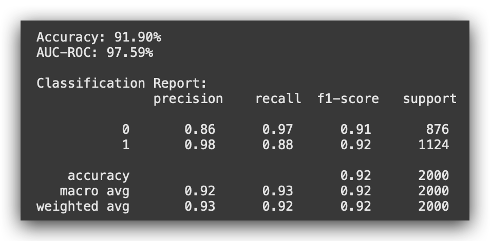
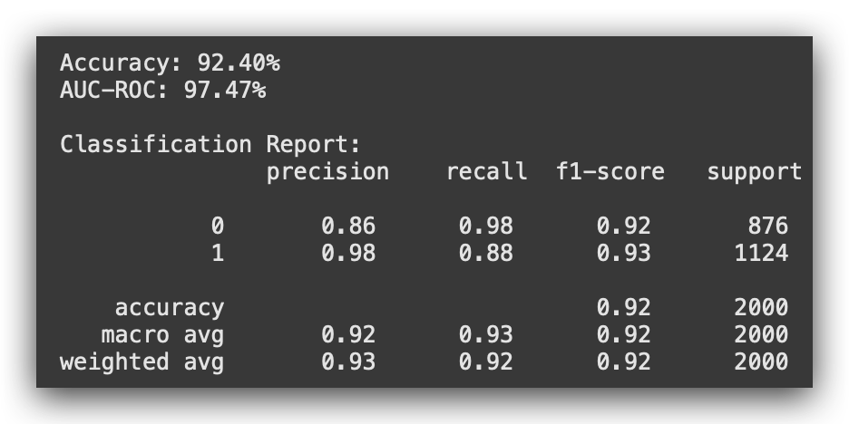
Now, I’ll show you the effect. Using LightGBM, you can already observe a noticeable drop in performance when the sequence is altered, can’t you?
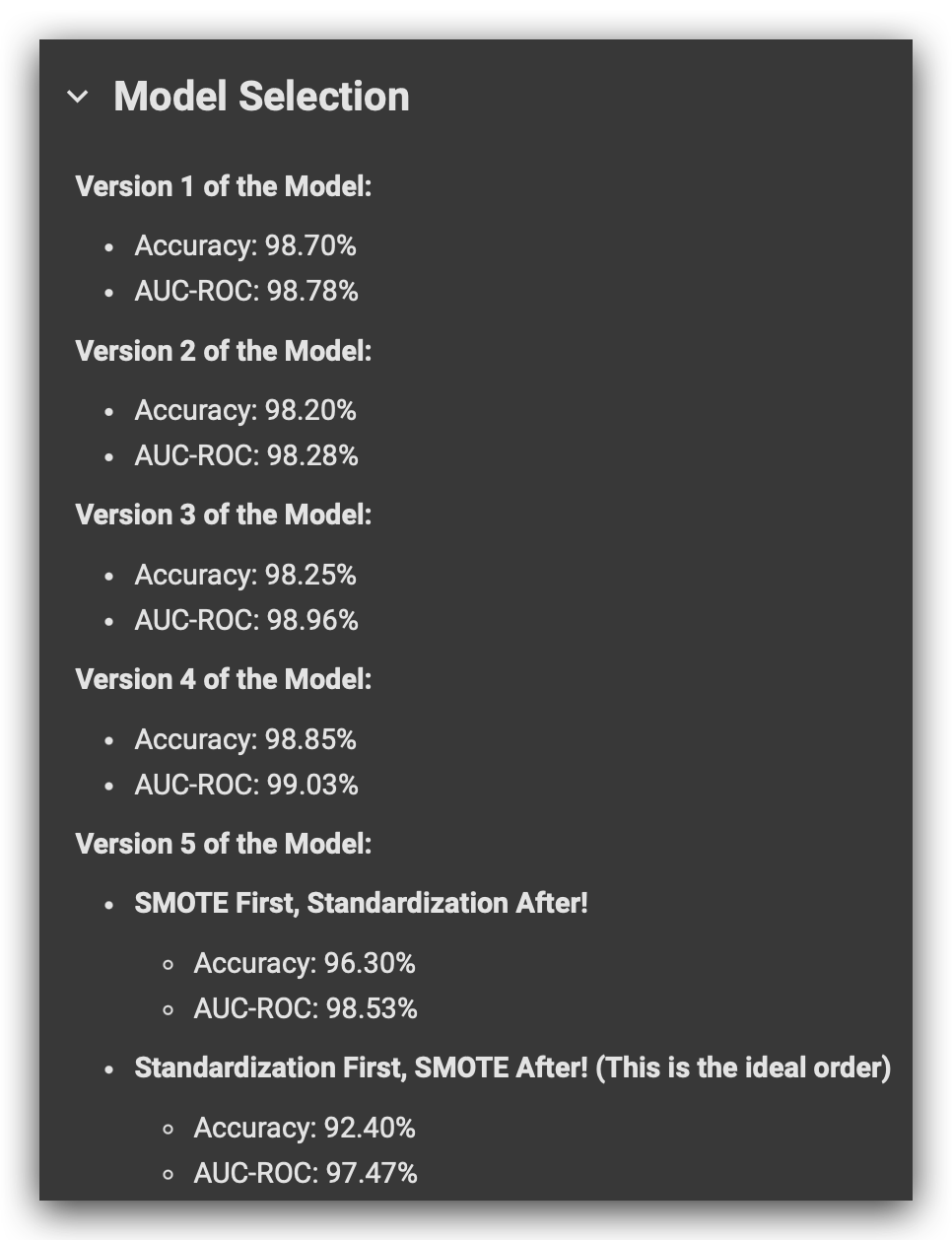
Let’s analyze version 5. With SMOTE applied first, we achieved an accuracy of 96.3% and an AUC-ROC of 98.53%. However, when we applied standardization first, the metrics dropped.
Why the discrepancy?
While standardization before SMOTE is the recommended approach, it doesn’t guarantee better results every time. Theoretically, standardizing first ensures more consistent distance calculations for SMOTE. However, applying SMOTE before standardization, although not ideal, was done here for demonstration purposes to highlight the difference.
Key conclusion for version 5
Using LightGBM, we observed significantly lower performance compared to Random Forest. This confirms that Random Forest, at least in this case, was already the better algorithm.
The switch to LightGBM caused a considerable drop in performance, proving that Random Forest was helping, not hindering.
While SMOTE-first might have yielded reasonable metrics, it’s not the recommended sequence. The results highlight that the earlier approaches (versions 1–4) were more effective.
With version 5, we can confidently conclude that Random Forest remains the optimal choice. I’ll now save this version for record-keeping, though the decision will be made among versions 1 to 4. Let’s proceed to save version 5.
# 67. Save the model and scaler to disk
model_file = 'model_v5.pkl'
scaler_file = 'scaler_v5.pkl'

joblib.dump(model_v5, model_file)
joblib.dump(scaler_v5, scaler_file)

print(f"Model saved at {model_file}")
print(f"Scaler saved at {scaler_file}")

Now, let’s talk about model selection.
Version 5, as we observed, showed a significant drop in performance, so it doesn’t make sense to proceed with it. My focus now shifts to choosing the best model among versions 1 to 4.
10. Which Model Would You Choose?
We’ve built five versions of the model. At this point, I’ll conclude the modeling phase and move to the next step: selecting the best model for deployment to address the problem we’ve been working on.
Is it mandatory to stop here? No. If you’re not satisfied with the performance, there are additional strategies to explore:
- Testing other algorithms.
- Hyperparameter optimization.
- Further refining the dataset.
For instance, we didn’t apply feature engineering in this project. Could that improve performance? There’s only one way to find out — experiment.
However, for the purpose of this example, our modeling work is sufficient.
When Do You Conclude the Modeling Phase?
Typically, we define a target metric at the start of the project. For instance:
- “When the model achieves 98.1% accuracy, we’ll use it in production.”
In our case, we’ve already surpassed 98.1% accuracy, so we can proceed to the next step.
If the goal were 99.7% accuracy, none of the versions met the criteria. In that case, we’d need to continue modeling.
For this project, we now move forward with model selection.

I’ve compiled the metrics for all five versions here again. It’s always good to rely on more than one metric because a single metric might not tell the whole story about the model’s performance. That’s why I’m presenting both Accuracyand AUC-ROC.
Now, here’s the big question: Which model would you choose?
Let’s start with Version 5. I think we can already discard it, right? We changed the algorithm while continuing to use SMOTE, but the performance dropped significantly. So, it doesn’t make sense to use Version 5 when we have models with better performance. That simplifies things a bit, doesn’t it?
Now, our choice is between Versions 1 through 4.
Our cutoff is 98.1% Accuracy. Any model achieving 98.1% or higher is considered acceptable. Based on this criterion, all four models qualify.
Wait a second, though. Are you saying performance alone can’t be the only criterion for choosing a model? Exactly! Excellent observation.
If performance isn’t enough, what other criteria should we consider?
1. Generalization Capability
A good model must generalize well, and this is often evident when the metrics are consistent across evaluations.
Looking at Versions 1 through 4, the metrics appear very close for each model. Perhaps Version 3 shows slightly more variation, but overall, all four models demonstrate strong generalization.
2. Interpretability
Interpretability is crucial when it comes to understanding and explaining a model’s predictions.
Among these four versions, there’s no difference in interpretability since all use the same Random Forest algorithm. It’s another tie.
3. Simplicity
This is the key differentiator. You want the simplest model possible.
Why? Complex models:
- Are harder to train.
- Are more challenging to deploy.
- Tend to be heavier and more resource-intensive.
- Are more prone to issues like model drift or data drift, where the model’s predictive capability deteriorates over time.
A simpler model is easier to maintain and less susceptible to these issues.
Which Version is the Simplest?
When comparing Versions 1 through 4, Version 1 is the simplest.
It directly handles class balancing at the model level without modifying the dataset, while the other versions introduce additional complexity with undersampling, oversampling, or SMOTE.
Final Choice
Considering performance, generalization, interpretability, and simplicity, Version 1 is the clear choice for deployment.
By selecting Version 1, we ensure a model that is robust, interpretable, and easy to deploy. Now, let’s move forward with this version!
11. Here’s the Main Model Selection Criterion
Take a moment to think about the models: Which one is the simplest, and why? And, most importantly, which model would you choose to deploy?
Remember, during deployment, the model will solve — or at least help solve — the business problem for which it was designed.
Your choice of model will directly impact the company’s results.
This means your decision must be grounded in clear and objective criteria.
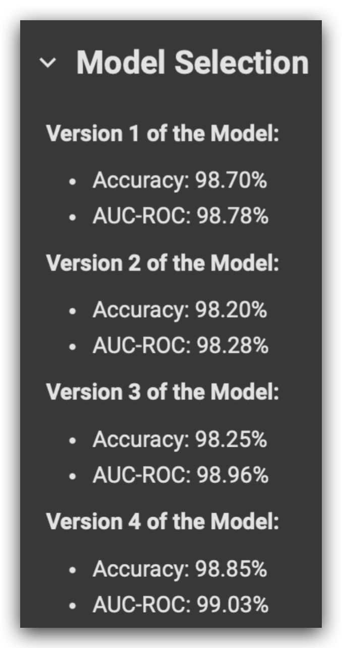
When considering these four model versions, there’s no wrong choice per se. All four are good models, demonstrating solid performance. Any of them, if deployed, would likely meet the business requirements.
However, one stands out as the best. It balances not only performance but also factors like simplicity, generalization capability, and interpretability.
Have you thought this through? A machine learning model is the result of this equation: Algorithm + Data. Never forget that. It’s not just about tweaking algorithm parameters. A model’s success depends on both the algorithm and the data.
A simple model is one that achieves strong performance with minimal changes to the data and minimal tuning of the algorithm. Based on this criterion, Version 1 emerges as the best choice for deployment.
Version 1 strikes the right balance between generalization capability, performance, simplicity, and interpretability. This balance is the essence of our task — finding a model that harmonizes these four factors, which is as much art as it is science.
In Version 1, I managed to address the class imbalance problem without altering the data. By fine-tuning an algorithm parameter, I achieved strong performance with minimal complexity. This makes it our optimal choice for deployment.

This parameter wasn’t used in the other options, right? But in Option 1, I didn’t need to modify the data. In other words, the impact on the model’s results was minimal. In all the other options, we made greater changes because we had to manipulate the data.
Is there a guarantee that you’ll always achieve good performance by adjusting a single parameter? No, there isn’t. This approach worked for this specific project, dataset, and algorithm — Random Forest. Tomorrow, I might work on another project with a completely different dataset, and in that case, the best model might require applying oversampling.
However, in our case, the simplest model is Version 1, which leads us to reflect on some important points. The less you alter the data, the better. By keeping the data intact, you preserve its essence — the information it carries. Each modification, in some way, impacts the data’s pattern. Every time you perform resampling — whether undersamplingor oversampling — you’re influencing the data, which adds complexity to the model.
You might argue, “But I had to manipulate the data.” And yes, when necessary, we do what’s required — alter, transform, and process the data. The goal is to find the best model, and that’s exactly what we’ve done here. Our best model is Version 1 because, given our current scenario, it’s the simplest model while the other criteria remain similar across versions.
Versions 2, 3, and 4 all involve transformations to the data. Whether by eliminating data through undersampling, creating synthetic data via oversampling, or using automated methods like SMOTE, these versions introduce additional complexity.
Considering all these criteria, Version 1 emerges as the best choice. It’s the simplest model while still offering strong generalization, performance, and interpretability. Done. Bingo. Checkmate. Version 1 is the model to move forward with for deployment.
If you arrived at a different conclusion, it’s essential to justify your choice. My answer isn’t the ultimate solution — it’s based on the science of machine learning. The simpler the model, the better. The less we manipulate the data, the better. The fewer changes made to the algorithm, the better.
The only model that aligns with all of this is Version 1. In the other versions, we altered the data. When that’s unavoidable, we make those transformations. However, Version 1 allowed us to achieve solid performance with the fewest possible changes to both the data and the algorithm.
For this reason, Version 1 is my choice, and this is the version we’ll now test in deployment.
12. Testing Model Deployment
We’ve made our decision, so now we can test the deployment.
This step is crucial as we’ll soon integrate it into the application we’re building with Streamlit.
To begin, we’ll create a function called maintenance_recommendation, which will accept new data as input.
# 68. Function to recommend maintenance based on new IoT sensor data
def maintenance_recommendation(new_data):

    # Define the column names as per the scaler adjustment
    columns = ['vibration', 'temperature', 'pressure', 'humidity', 'working_hours']

    # Convert new data to DataFrame with correct column names
    new_data_df = pd.DataFrame([new_data], columns=columns)

    # Apply the scaler to the new data
    new_data_scaled = scaler_v1.transform(new_data_df)

    # Make the prediction
    prediction = model_v1.predict(new_data_scaled)

    if prediction == 1:
        return "Recommendation: Perform maintenance."
    else:
        return "Recommendation: No maintenance needed."
I will define the column names for the input data.
This data will then be converted into a DataFrame, and I’ll assign the column titles to a DataFrame named new_data_df.
What needs to be done with the new data? Standardization.
Every transformation applied to the training data must also be applied to the test and new data. For this, I’ll use scaler_v1, as it’s the standardizer for model_v1, our selected model.
Once the data is standardized, it’s passed to the model for class prediction. If the prediction is 1, maintenance is required. Otherwise, it’s not.
Let’s define this function. I’ve prepared a new dataset to test it:
# 69. Example of new IoT sensor data
new_data_1 = [0.5, 80, 102, 45, 8000]
print(maintenance_recommendation(new_data_1))

# -----> Recommendation: Perform maintenance.

# 70. Example of new IoT sensor data
new_data_2 = [0.89, 92, 96, 70, 600]
print(maintenance_recommendation(new_data_2))

# -----> Recommendation: No maintenance needed.
The first IoT sensor reading indicates that the machine requires maintenance. This is the recommendation.
For the second reading below, for instance, no maintenance is required.
Great! The model has been successfully tested and is ready. Now we can proceed to deploy it using Streamlit.
13. Deploying the Model with Streamlit
To wrap up our project on a high note, let’s deploy the model!
It’s important to note that deploying a model isn’t usually the responsibility of a data scientist.
In most cases, particularly in many companies, deployment is handled by Machine Learning Engineers, as deployment involves its own specialized set of skills and practices.
That said, since we’re here, let’s take the opportunity to create an app using Streamlit for deploying the model.
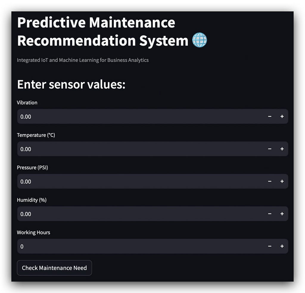
To start, I’ll run the app so you can see its interface — which is quite user-friendly! Simply execute the following via the command line.
Open your terminal or prompt, navigate to the directory where your files are saved, and copy the full path. For example, in my case, it’s:
cd ~/Documents/Projects/recommendation_project
To execute Streamlit, follow these steps:
- Open your terminal or command prompt.
- Type the command to indicate you want to run Streamlit.
- Specify what you want to do: in this case, use run to execute.
- Finally, include the name of the script file.
streamlit run recommendationapp.py
Just press Enter in the terminal or command prompt, and that’s it! The app will start loading.
Wait a few moments, and voilà — our Streamlit app for deployment will be up and running, ready for use. 🎉
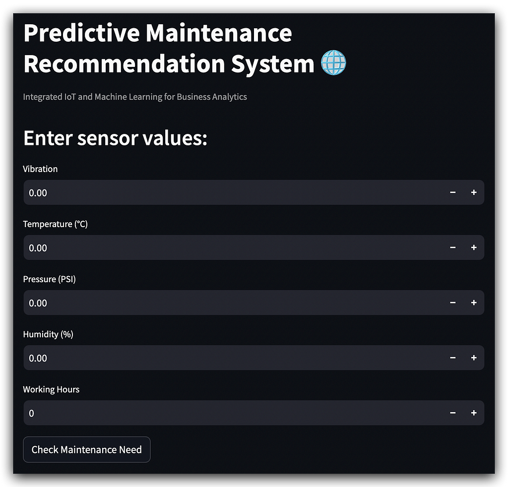
There’s a main title, followed by what Streamlit refers to as a caption, which is essentially a smaller explanatory text.
Then we have a subtitle guiding the user on what to do: input the necessary data.
Once the user finishes entering the input values, they press the Check Maintenance Need button, and the magic happens.
A quick reminder: while running the app, you’ll need to keep the terminal open for everything to function properly.
Now, let’s move on to the execution. Here are some sample values to input:
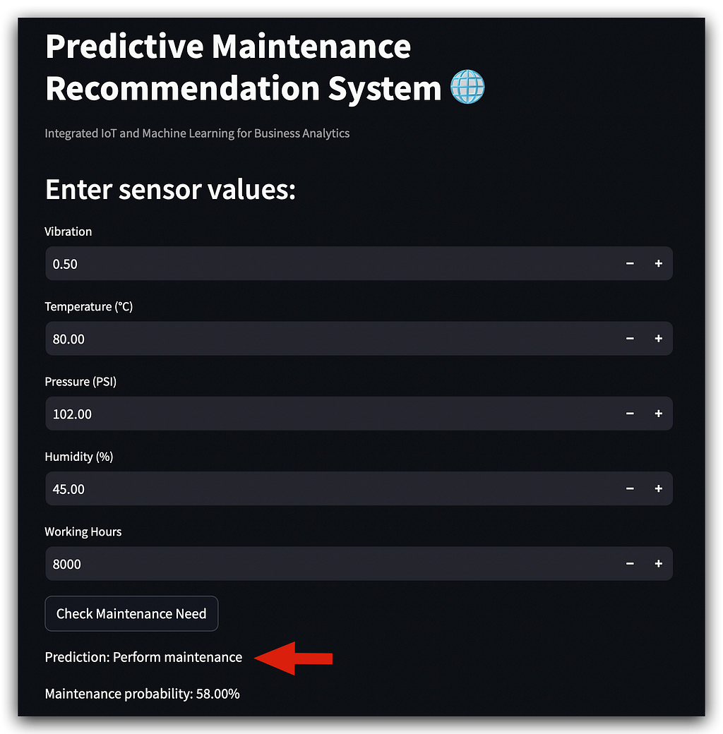
Click the Check Maintenance Need button, and yes, it indicates maintenance is required with a probability of 58%.
Beyond that, there’s not much more to add, right?
We’re delivering a complete recommendation system, including the probability of maintenance or not.
It’s not just a simple yes or no answer; the app provides the probability.
For instance, if you have two machines requiring maintenance, you can prioritize the one with a higher probability. This feature adds depth to the system, giving valuable insights through our app for deployment.
Let’s test another example. Simply modify one input value, and it will reset the output.
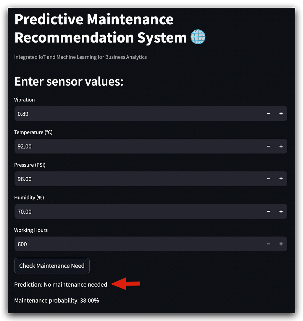
In this configuration, no maintenance is necessary, with a probability of 38%.
You know the model provides probability predictions, right? So, relying solely on a yes or no can be risky. If we left it at that, it would simply say no, but notice that this no comes with a 38% probability.
Perhaps we could introduce a filter, for instance, to give the company more confidence when deciding whether or not to proceed with maintenance.
# 69. Example of new IoT sensor data
new_data_1 = [0.5, 80, 102, 45, 8000]
print(maintenance_recommendation(new_data_1))

# -----> Recommendation: Perform maintenance.

# 70. Example of new IoT sensor data
new_data_2 = [0.89, 92, 96, 70, 600]
print(maintenance_recommendation(new_data_2))

# -----> Recommendation: No maintenance needed.
You can see that I used the exact same values as before.
The model must be consistent when delivering results, as is required in our recommendation system.
14. Building the App
Let’s now look at how to build our app using the script recommendationapp.py.
Open your text editor, and here is the complete script:
# Predictive Maintenance Recommendation System Integrated with IoT to Reduce Unplanned Downtime

# Imports
import joblib
import streamlit as st
import numpy as np
import pandas as pd

# Load the saved model and scaler
model_file = 'models/model_v1.pkl'
scaler_file = 'scalers/scaler_v1.pkl'
model = joblib.load(model_file)
scaler = joblib.load(scaler_file)

# Function to make maintenance recommendations
def maintenance_recommendation(new_data):
    # Define column names as per the scaler
    columns = ['vibration', 'temperature', 'pressure', 'humidity', 'working_hours']

    # Convert the new data into a DataFrame with correct column names
    new_data_df = pd.DataFrame([new_data], columns=columns)

    # Apply the scaler to the new data
    new_data_scaled = scaler.transform(new_data_df)

    # Make predictions
    prediction = model.predict(new_data_scaled)
    prediction_proba = model.predict_proba(new_data_scaled)[:, 1]

    # Return the predicted class and probability
    return prediction[0], prediction_proba[0]

# Configure the Streamlit app page
st.set_page_config(page_title="Predictive Maintenance System", page_icon="⚙️", layout="centered")

# Define the app title
st.title("Predictive Maintenance Recommendation System 🌐")

# Define an explanatory caption for the app
st.caption("Integrated IoT and Machine Learning for Business Analytics")

# Input header
st.header("Enter sensor values:")
vibration = st.number_input("Vibration", value=0.0)
temperature = st.number_input("Temperature (°C)", value=0.0)
pressure = st.number_input("Pressure (PSI)", value=0.0)
humidity = st.number_input("Humidity (%)", value=0.0)
working_hours = st.number_input("Working Hours", value=0)

# Button to make a prediction
if st.button("Check Maintenance Need"):
    new_data = [vibration, temperature, pressure, humidity, working_hours]
    prediction_class, prediction_probability = maintenance_recommendation(new_data)

    # Display results
    st.write(f"Prediction: {'Perform maintenance' if prediction_class == 1 else 'No maintenance needed'}")
    st.write(f"Maintenance probability: {prediction_probability:.2%}")
To build the app, we need to capture user input, process it, and display the model’s predictions. Below is a streamlined explanation of the process:
Input and Processing
- The app collects user inputs via a form.
- These inputs are processed into a Pandas DataFrame, standardized using scaler_v1 (specific to model_v1), and passed to the prediction model.
- Predictions include both the class (e.g., maintenance required or not) and the probability.
Streamlit Interface
- Use Streamlit to create an interactive UI:
- Title, captions, and number input fields for predictive variables.
- Default values for the form fields are set to 0.
- When the user clicks the button, the inputs are sent to the function maintenance_recommendation, which returns predictions.
Model Loading
- Load model_v1 and scaler_v1 from disk into memory. These are critical for processing new data and making predictions.
Enhancements
- The maintenance_recommendation function now includes probability predictions.
- Display both the class and probability on the app, allowing better decision-making.
Script Highlights
- st.number_input creates input fields.
- The button triggers an action captured by an if block, processing the inputs through the prediction function and returning the results.
- Results include “Maintenance Required” or “No Maintenance Needed” with probabilities rounded to two decimal places.
Conclusion
- The app is fully functional and ready for deployment.
- Future enhancements could include a history of predictions, charts for trends, or additional user interface features.
Final Notes
This approach ensures an intuitive app that provides accurate recommendations based on IoT data, completing the project and deployment successfully.
15. Conclusion
Building a professional-level data science project is far from easy, despite what some might claim. If anyone tells you otherwise, they likely don’t understand the complexity involved. As demonstrated, this process goes well beyond simply writing Python code.
A data science project is a multifaceted endeavor that requires much more than scripting. It involves understanding the business problem, selecting the right tools, interpreting results, and making critical decisions at every stage.
For example, choosing the right model was a significant step in this project. Additionally, we went beyond modeling by creating a deployable application, showcasing the level of effort and expertise required for a truly professional outcome.
This project emphasized two key aspects: modeling and effectively managing imbalanced data. While not every possible strategy was explored, that was intentional.
Each project I work on highlights specific techniques or concepts. In this case, the focus was on addressing imbalanced data, but real-world scenarios often demand combining various strategies within a single project.
You’re encouraged to take this tutorial further. Experiment with feature engineering, try out different models, adjust algorithms, or perform hyperparameter tuning to refine the results. By modifying and expanding upon this foundation, you might achieve even better performance than demonstrated here.
In the end, constructing a project like this is a journey filled with challenges and learnings — but the payoff is worth the effort.
Below are the key references and resources used throughout this project, along with additional materials to deepen your understanding:
16. Bibliography, References, and Useful Links
- Imbalanced-learn Documentation
Guide for handling imbalanced datasets.
Imbalanced-learn Official Site - LightGBM Documentation
Detailed reference for the LightGBM algorithm.
LightGBM Official Site - Streamlit Documentation
A complete guide to building interactive web apps for ML models.
Streamlit Official Site - GitHub Repository
Access the complete project code, datasets, and resources.
GitHub - Anello92/Preventive-Maintenance-Recommendation-System-
Thank you, as always! 🐼❤️
All images, content, and text by Leo Anello.
Predictive Maintenance Models with a Focus on Class Balancing — Complete Notebook was originally published in Towards Data Science on Medium, where people are continuing the conversation by highlighting and responding to this story.
from Datascience in Towards Data Science on Medium https://ift.tt/tFi3ZLl
via IFTTT


