Satellite Image Classification Using Deep Learning | By Leo Anello | Medium
Learning Image Classification with Deep Learning
A Step-by-Step Approach Using Satellite Data
Project Overview
This tutorial is part of a series where I’ll explore deep learning applications across various domains, each with its own project.
The focus here is on learning deep Learning and image classification.
We could have chosen to classify cats, dogs, or flowers, but for this project, we opted to work with satellite images as they provide a unique and exciting challenge.
For this, we’ll use the EuroSAT_RGB dataset, generously shared by my friend Blanchon on Hugging Face. A special thanks to him for making this dataset available to the community, enabling projects like this.
In this case, the goal is to teach a model to categorize different types of environments — like forests, rivers, or urban areas — based on satellite imagery.
However, the potential applications of this type of technology extend far beyond satellite images, including:
- Medical imaging, like detecting tumors in X-rays or MRIs.
- Autonomous vehicles, enabling them to recognize roads, obstacles, and pedestrians.
- Retail, for customer behavior analysis through video footage.
- Agriculture, identifying crop health or monitoring irrigation patterns.
- Environmental monitoring, like tracking deforestation or air pollution.
This project is not just about solving a satellite-specific problem but also about learning to apply deep learning techniques in practical scenarios
By the end of this tutorial, you’ll have built a functional model, understood the fundamentals of computer vision, and gained skills that can be applied to other real-world challenges.
The complete project files and notebook will be available on my GitHub:
If you enjoy this project, your support is always welcome — every bit helps!
Imagine the following scenario:
You’re playing soccer with a friend. They throw the ball, and you catch it with your hands. It seems simple, right? Wrong.
This is one of the most complex processes we’ve ever tried to understand. How does the brain process vision so we recognize a ball and predict its trajectory?
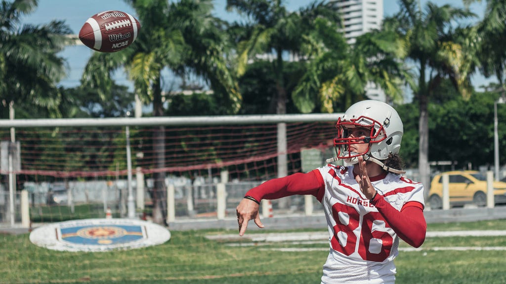
Have you ever thought about this? Look at an object near you — perhaps the phone you’re using to read this tutorial. In a fraction of a second, the image of that object passes through your eye, engages muscles, reaches your brain, accesses stored knowledge, and returns an understanding.
This process allows you to recognize the object, decide on an action, and execute it — all in milliseconds. Let’s briefly describe this process. Using the example of catching a thrown ball, we’ll simplify how human vision works.
The image of the ball passes through your eye and hits your retina, where some elementary analysis occurs. The result is sent to your brain, where the visual cortex performs a deeper analysis. It then communicates with other parts of the cortex, comparing stored knowledge, classifying objects and dimensions, and deciding on an action.
For example, it predicts the ball’s trajectory, tells you to raise your hand, and catch it. All of this happens in a fraction of a second, requiring almost no conscious effort and rarely failing. This is human vision. But someone thought, “Wow, this is fascinating — can we replicate it in computers?”
And how do we replicate this process in machines? For now, there’s only one answer: mathematics. Yes, once again, math provides the solution to replicate human vision in machines. This brings us to the question: What is computer vision?
Computer vision is the mathematical modeling of human vision using software and hardware. While it doesn’t fully replicate human vision, it works well for many use cases. For instance, it can classify or segment images, detect objects in real-time videos, and much more.
It’s far from matching human vision, but that’s not the goal. The objective is to build applications that enable computers to work with images and videos, which is increasingly common in our daily lives.
2. Satellite Image Classification with Deep Learning
This project focuses on building a deep learning model from scratch to classify satellite images — a typical example of a computer vision project.
We’ll use the dataset available at the following link:
blanchon/EuroSAT_RGB · Datasets at Hugging Face
The data is compressed into a ZIP file, which you can download here:
Our goal is to build a deep learning model for satellite image classification.
To achieve this, we’ll explore one of the most important architectures in Deep Learning today: convolutional neural networks (CNNs).
Almost any Deep Learning project in computer vision involves convolution operations. Understanding how CNNs work is crucial.
In this project, we’ll construct the entire architecture from scratch and train the model from the ground up. I won’t use pre-trained models here. This approach will help you develop the skills needed to build models entirely from scratch.
Since we’ll be training the model on a substantial volume of images, we’ll need a GPU for efficiency.
To make this accessible, we’ll use Google Colab, a cloud platform that provides free access to GPUs.
3. Organizing Files
Let’s start the project by organizing the files in Google Colab. Why use Google Colab? Because of the GPU it provides, which significantly speeds up the training of deep learning models. Training time can drop from 3–4 hours to just 10–15 minutes.
Using a GPU isn’t mandatory, but let’s be honest: faster training is always better. If you have a computer with a compatible GPU, you can use it as well. Just ensure you install the CUDA platform and confirm that your GPU supports the required Compute Capability.
If compatibility issues arise, stick with Colab. It’s free, easy to use, and comes with built-in GPU support. To get started, download the notebook from my GitHub (linked at the end of the tutorial). Upload it to Colab by dragging the file into the interface.

Select Runtime, then click on Change Runtime Type.
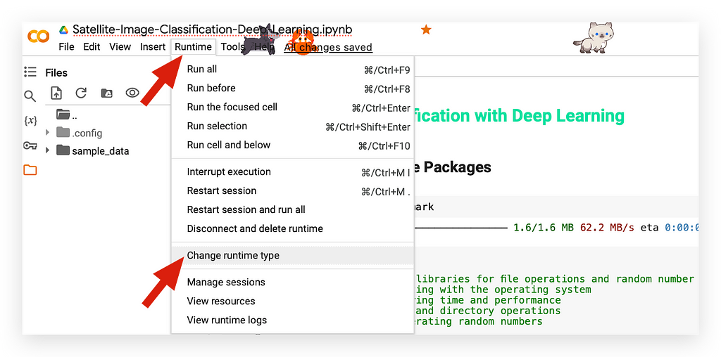
The free version provides access to the T4 GPU, which is part of the free tier. Using only a CPU doesn’t make sense here — I want to utilize the GPU.
Now, I need to upload the zip file containing the images. Inside the images folder, you’ll find this zip file with the original data.
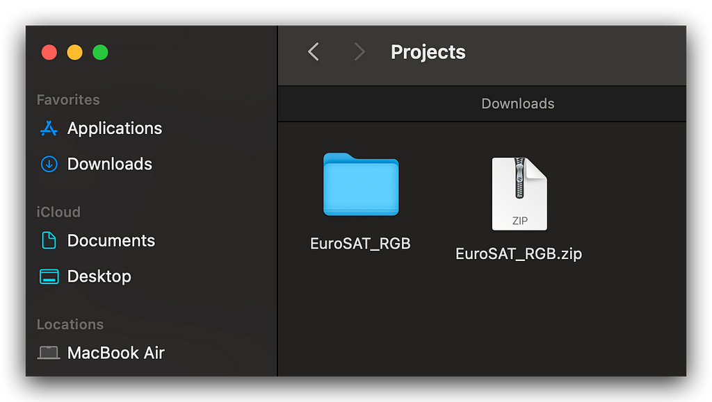
This is the dataset containing satellite images. The file size is over 100 megabytes. Download it using the link I provided from Google Drive and save it to your machine.
Next, take the zip file and drag it into the Files section of Colab. Simply drag and drop the zip file.
You’ll see a message indicating that once the session expires or if you delete your runtime, all files uploaded here will be lost. Keep this in mind.
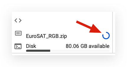
Notice that, at the bottom, it shows the file is currently being uploaded. There’s a blue line in a circle, indicating the progress of the upload.
Once complete, the zip file will be ready.
In the notebook, I’ve already included the commands to unzip the file, prepare the directory, and then train your model.
Everything is set up for you. Your task is to upload the notebook, upload the zip file, and follow along with this amazing project.
4. Installing and Loading Packages
Let’s begin executing the notebook by installing the watermark package:
!pip install -q -U watermark
Next, we’ll load the necessary packages for our work:
# 1. Imports

# 1.a Importing standard libraries for file operations
import os      # For interacting with the operating system
import time    # For measuring time and performance
import shutil  # For file and directory operations
import random  # For generating random numbers

# 1.b Importing numerical and visualization libraries
import numpy as np               # For numerical operations and array manipulation
import seaborn as sns            # For statistical data visualization
import matplotlib.pyplot as plt  # For plotting and visualizations

# 1.c Importing PyTorch libraries for deep learning
import torch                                 # Core PyTorch library
import torchvision                           # For datasets and pretrained models
import torchvision.transforms as transforms  # For data augmentation and transformations
from torchvision.datasets import ImageFolder # For loading image datasets organized in folders

# 1.d Importing PyTorch modules for building and training neural networks
import torch.nn as nn            # For defining neural network layers
import torch.nn.functional as F  # For activation functions and other utilities
import torch.optim as optim      # For optimization algorithms

# 1.e Additional tools for progress visualization and evaluation
from tqdm import tqdm                         # For creating progress bars
import sklearn                                # For machine learning utilities
from sklearn.metrics import confusion_matrix  # For calculating the confusion matrix
The os package will be used to manage files and directories on the disk, including images and folders. It's the Operating System package, and I'll rely on it for these tasks.
The time package will help measure execution time.
I'll also use shutil, which, as the name suggests, is very handy. With this package, I can handle operations such as deleting an entire folder if it exists.
For example, if I want to remove a folder and all its contents, shutil makes it easy. You might be wondering, "Why would I need to delete an entire folder? Can't I just right-click and delete it like in Windows?" Well, it's not quite the same.
For instance, take a look at this folder named sample_data:
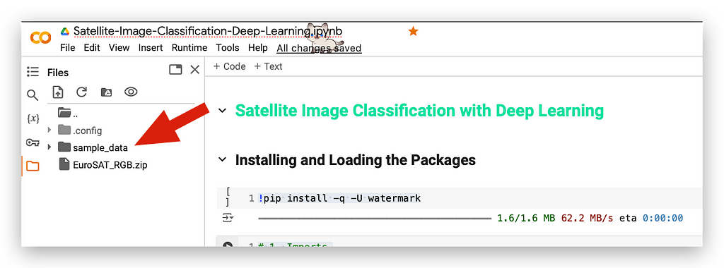
This folder contains files from Colab. Every time you use Colab, these files are present. Now, let’s say I want to delete this folder.
You can click on the three dots next to it, select Delete Folder, and then confirm when prompted. Simply click OK, and the folder will be removed.
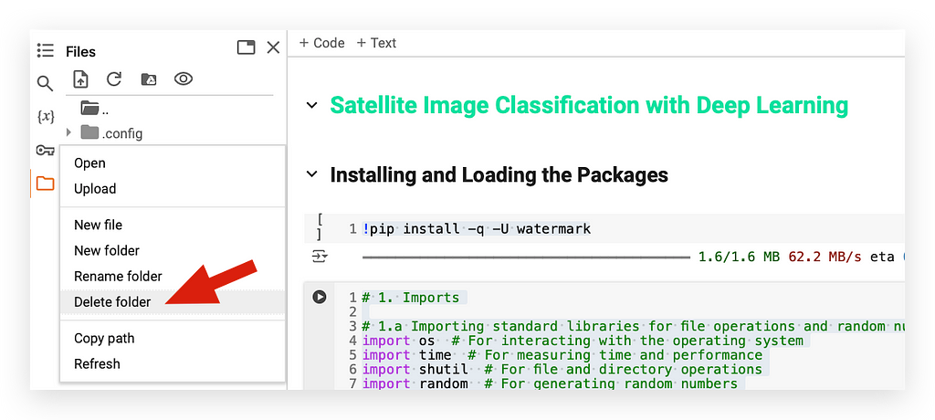
Notice that the deletion failed. Now, take a look at the message displayed:
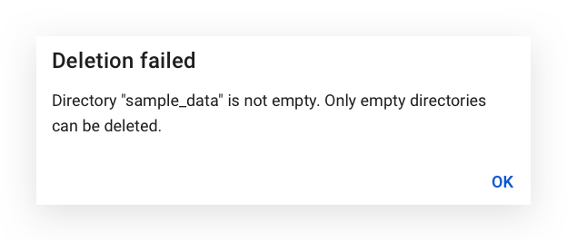
The directory isn’t empty. Only empty directories can be deleted.
When I unzip the zip file, it will generate several images across various folders. Later, I’ll create our directories. If I need to rerun the notebook, I won’t be able to execute it properly with the existing directories, as this will cause conflicts.
You’ve already seen what happens when I try to delete a folder manually — it doesn’t work. That’s why I need rmtreefrom the shutil module.
This command deletes an entire directory, including all its contents, allowing me to run the notebook as many times as I want without needing to manually remove files.
Pretty useful, right? Using this tip in Colab is fantastic. I could now, for example, go to Runtime and select Run All to execute everything seamlessly.
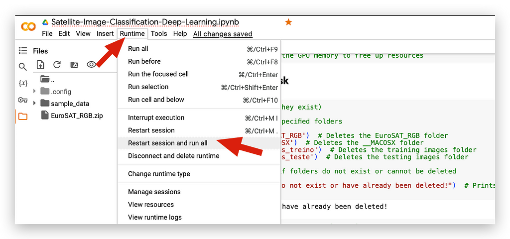
If an error occurs and I need to change a parameter, all I have to do is go to Runtime, restart the session, and run everything again.
There’s no need for additional manual steps because my script is already set to handle directories.
It deletes existing folders, recreates them, and gets everything ready without requiring me to perform these tasks manually. Isn’t shutil an amazing package?
We’ll also use the random package to generate random values when needed. NumPy is essential for working with matrices—since an image is essentially a matrix of pixels. With multiple images, we’ll be handling several pixel matrices, and NumPy is perfect for this.
For visualization, we’ll use Seaborn and Matplotlib to generate graphs.
For constructing our Deep Learning model, we’ll rely on torch from the PyTorch framework. PyTorch is one of the leading frameworks for deep learning, enabling us to build and train model architectures effectively.
However, we’ll also need to process and transform the input images — similar to how you preprocess text files or Excel sheets. For this, we’ll use TorchVision, a PyTorch library dedicated to image transformations. It allows us to preprocess images, apply transformations, and prepare datasets.
From TorchVision, we’ll use ImageFolder to organize our image directories. Additionally, we’ll implement tqdm to display a progress bar while training the model, as this process takes some time. This progress bar will ensure everything is running as expected.
Finally, we’ll use Scikit-Learn to generate a confusion matrix as part of the model’s performance metrics.
Don’t forget to execute this cell to load the Watermark package:
%reload_ext watermark
%watermark -a "Your_Name_Here"
I’ll check the hardware being used.
It’s already displayed above that I’m using the A100 GPU, but with this code snippet, I can verify the type of GPU in use:
# 2. Check the GPU model

# 2.a Verify if a GPU is available
if torch.cuda.is_available():
    # 2.a.1 Print the number of GPUs available
    print('Number of GPUs:', torch.cuda.device_count())

    # 2.a.2 Print the model name of the first GPU
    print('GPU Model:', torch.cuda.get_device_name(0))

    # 2.a.3 Print the total GPU memory in GB
    print('Total GPU Memory [GB]:', torch.cuda.get_device_properties(0).total_memory / 1e9)
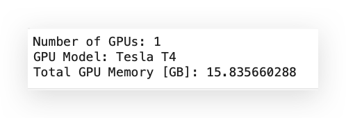
When we execute the code, we can confirm that there is a single Tesla T4 GPU with 16 GB of memory — fantastic!
If at any point the GPU memory fills up too quickly, you can use Numba, a Python package, to reset the GPU memory. Here’s the code snippet:
# 3. Reset GPU memory

# 3.a Import the required library for GPU memory management
# Provides tools to interact with NVIDIA GPUs
from numba import cuda

# 3.b Get the current GPU device
# Retrieves the current active GPU device
device = cuda.get_current_device()

# 3.c Reset the GPU memory
# Clears the GPU memory to free up resources
device.reset()
When needed, you can perform this action without having to close and reopen everything, making our workflow much smoother.
Now that we have all the necessary packages, let’s proceed to organize the images on disk.
5. Organizing Images on Disk
We will now extract the contents of the zip file.
Everything is automated for you directly in the Jupyter Notebook using Python code. First, we have a try-except block:
# 4. Delete folders (if they exist)

# 4.a Attempt to remove specified folders
try:
    shutil.rmtree('EuroSAT_RGB')      # Deletes the EuroSAT_RGB folder
    shutil.rmtree('__MACOSX')         # Deletes the __MACOSX folder
    shutil.rmtree('training_images')  # Deletes the training images folder
    shutil.rmtree('testing_images')   # Deletes the testing images folder

# 4.b Handle exceptions if folders do not exist or cannot be deleted
except Exception as e:
    # Print an error messagean error message
    print(f"The folders do not exist or have already been deleted!")
When you unzip the file, it will automatically create the EuroSAT_RGB folder along with a MACOSX folder, which is included by the creators of the zip file. After that, we’ll create training_images and testing_images.
During the first execution, none of these folders will exist yet. Starting from the second execution of the Jupyter Notebook, the folders will already be there. At that point, the try block will execute, removing the folders, and you'll be able to run the entire notebook in an automated manner.
This approach lets you automate the process and execute the entire notebook without manual intervention. Now, let’s unzip the file — you won’t believe the command we’re about to use:
# 5.a Extract the EuroSAT_RGB.zip file

# Unzips the file into the current directory
!unzip EuroSAT_RGB.zip
Because now it’s Linux! Colab operates in a Linux environment, where everything just works. All you need to do is use the unzip command. It’s a system command, so you add an exclamation mark (!) before it.
Run the command, cross your arms, and wait. The zip file will be extracted. Notice how it creates the _MACOSX folder, which is likely a cache folder left over from the machine used to prepare the dataset.
Once the extraction is complete, take a look at how it created the folders:
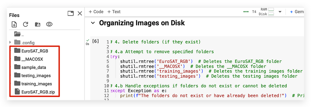
The _MACOSX folder is just a cache directory, while the EuroSAT_RGB folder contains the actual data. If you click on the arrow next to it, you'll see that there’s a folder for each category:
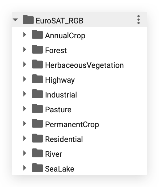
These are the categories I’ll train my model on shortly for classification.
When provided with a new satellite image, the model will be able to classify it into one of these categories.
This project, in essence, is a multiclass classification problem.
# 6. Create folders

# 6.a Create a folder for training images
os.mkdir('training_images')  # Creates the 'training_images' directory

# 6.b Create a folder for testing images
os.mkdir('testing_images')  # Creates the 'testing_images' directory
Notice that I’m automating this process with Python code. Sure, you could manually right-click and select “New Folder,” but there’s no need for that.
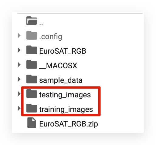
Using the os package and its mkdir function, which works seamlessly in this Linux environment, the command mkdir is executed. After refreshing, you'll see the training and testing folders have appeared, ready to use.
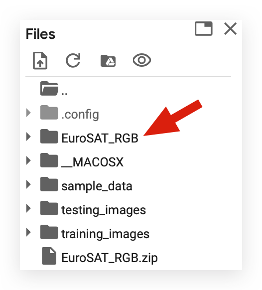
After that, I’ll define the variable images_source, which refers to the folder located above:
# 7. Define the source directory

# 7.a Set the source folder for the images
# Specifies the folder containing the source images
images_source = 'EuroSAT_RGB'
And then the destination, which will be the training_images and testing_images folders:
# 8. Define the destination directories

# 8.a Set the destination folder for training images
training_destination = 'training_images'

# 8.b Set the destination folder for testing images
testing_destination = 'testing_images'
With this setup, I already have the folders and the corresponding Python variables properly defined.
Now, I can automate the process of separating the images. I’ll iterate through the EuroSAT_RGB folder, split the images, and move them into the training_images and testing_images folders.
This will enable us to visualize the images later and, further ahead, train our model effectively.
6. Automating the Image Separation
Now, let’s see how to automate the process of separating the images. First, I’ll define a variable image_class with an initial value of 0.
This will be used as a control variable. Additionally, I'll create an empty dictionary called class_dictionary, which will serve to manage the automation process in the subsequent steps.
# 9. Class variable and dictionary

# 9.a Initialize the class variable
# Used to assign a class ID to each category of images
image_class = 0

# 9.b Initialize the class dictionary
# Stores the mapping of class IDs to class names
class_dict = {}
I will create a variable named files, which will be used to handle the images.
This variable will help manage the image files during the automation process.
# 10. Create a variable to manage the files

# 10.a List all files in the source directory
# Retrieves the list of files in the source folder
files = os.listdir(images_source)

# 10.b Sort the files alphabetically
# Ensures the files are processed in a consistent order
files.sort()
And then, I have a loop. Let’s take a look at what this loop does:
# 11. Iterate over all files (or directories) in the 'files' list
for file_path in files:

    # 11.a Check if the file (or directory) name does not start with a dot (not hidden)
    if file_path[0] != '.':

        # 11.b List all images in the specified directory
        images = os.listdir(images_source + '/' + file_path)

        # 11.c Calculate the sample size for the training set (80% of total images)
        sample_size = int(len(images) * 0.8)

        # 11.d Initialize an empty list to store the names of training images
        train = []

        # 11.e Define the final destination for the training images
        final_dest = training_destination + '/' + str(image_class)

        # 11.f Create a new directory for the training images
        os.mkdir(final_dest)

        # 11.g Select a random sample of images for the training set and copy them to the final destination
        for file_name in random.sample(images, sample_size):

            # 11.g.1 Copy the image to the destination directory
            shutil.copy2(os.path.join(images_source, file_path, file_name), final_dest)

            # 11.g.2 Add the image name to the training list
            train.append(file_name)

        # 11.h Get the list of images not selected for training (testing images)
        test_images = list(set(images) - set(train))

        # 11.i Define the final destination for the testing images
        final_dest = testing_destination + '/' + str(image_class)

        # 11.j Create a new directory for the testing images
        os.mkdir(final_dest)

        # 11.k Copy all testing images to the destination directory
        for test_image in test_images:
            shutil.copy2(os.path.join(images_source, file_path, test_image), final_dest)

        # 11.l Map the image class to its corresponding file path in the 'class_dict' dictionary
        class_dict[image_class] = file_path

        # 11.m Increment the image class identifier
        image_class += 1
Loop file_path in files: First, let's see what these files are about.
files
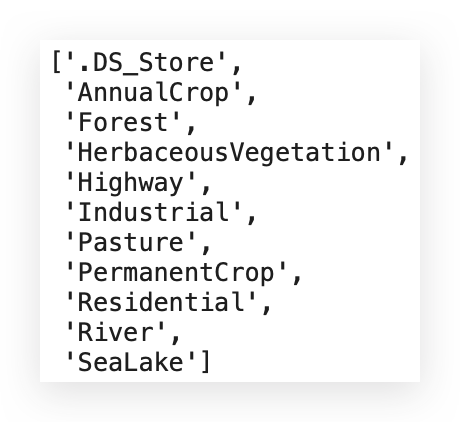
These are the files, which are essentially folders. I’ll navigate into each of these folders sourced from images_source, and for each of them, I will perform specific operations.
Again, within the loop file_path in files: if the file path is not a dot (meaning it's not the current directory), I'll list the images in the directory and calculate the sample size for the training set, using 80%.
I’ll then initialize an empty list and define the final destination. After that, I print the path and create a new directory using os.mkdir(final_dest). Next, I will select a random sample of images.
To summarize, I will randomly fetch images from the source folder, which, as mentioned earlier, is the EuroSAT_RGBdirectory.
Randomly, I'll retrieve images from this location.

To distribute the images into training and testing sets, I’ll use shutil.
Specifically, I’ll utilize shutil.copy2. This function allows me to copy files from the images_source, taking into account the file path and name.
# 11.g.1 Copy the image to the destination directory
            shutil.copy2(os.path.join(images_source, file_path, file_name), final_dest)
I’ll copy the images to final_dest, which represents the destination. In this case, the destination will be either training_images or testing_images.
The process involves copying the image—meaning the original image remains in its source folder. I’ll select the images randomly and transfer them to the destination.
This is implemented as a loop, right?
# 11.g Select a random sample of images for the training set and copy them to the final destination
        for file_name in random.sample(images, sample_size):

            # 11.g.1 Copy the image to the destination directory
            shutil.copy2(os.path.join(images_source, file_path, file_name), final_dest)

            # 11.g.2 Add the image name to the training list
            train.append(file_name)
Inside this loop, the process continues until I’ve allocated all the images — 80% of them, in this case — to the training set.
Next, I’ll prepare the testing images. Everything that went to the training set will be excluded, subtracted from the total. Whatever remains will be separated into the testing set.
I’ll define the final path, the destination, create the folder, and then iterate through another loop.
Similarly, I’ll copy the remaining images to final_dest.
I’ll add the file paths to the respective directories and increment the loop to proceed to the next folder, and so on.
When you execute the entire block, it will take a few moments to process. Shall we take a look? Enter the training_images folder:
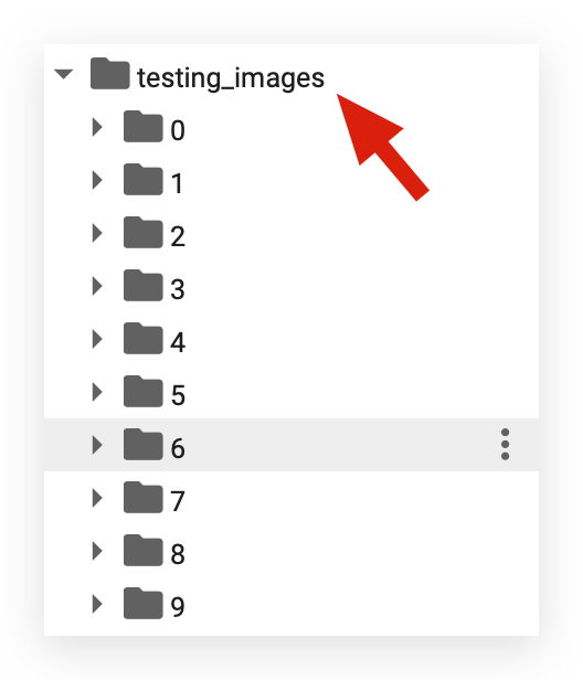
I have assigned a number to each class, which is why I started with 0 earlier. Starting from 0, we go up to class 9. How many classes do we have?
Ten in total. I no longer need to use the names, right? Now, I can work directly with the numbers.
Each number corresponds to an associated name here:

I want to represent the associated name mentioned above.
Inside each of these numbered folders, we now have the images that will be used for training. The same applies to the images designated for testing.
Therefore, I started by checking if those initial folders exist:
# 4. Delete folders (if they exist)

# 4.a Attempt to remove specified folders
try:
    shutil.rmtree('EuroSAT_RGB')
    shutil.rmtree('__MACOSX')
    shutil.rmtree('training_images')
    shutil.rmtree('testing_images')

# 4.b Handle exceptions if folders do not exist or cannot be deleted
except Exception as e:
    print(f"The folders do not exist or have already been deleted!")
If they exist, I delete them. Now everything is in place. If I execute it again, it will delete everything. After that, I decompress the zip file:
# 5. Extract the EuroSAT_RGB.zip file
# Unzips the file into the current directory
!unzip EuroSAT_RGB.zip
Decompressed. You create the necessary folders and define the Python variables. Then, you establish the control variables, enter the loop, and randomly select images from the source.
These images are distributed to the training and testing destinations, replacing the class names with their corresponding indices. This method ensures the preparation of input images.
Now, we’re ready to move on to the preprocessing step and create the dataloaders.
7. Project 3 — Preprocessing and Dataloader Creation
Now, we’ll preprocess the data and create the dataloaders. At this point, the images are stored on disk as files. The next step is to apply transformations so we can load these images and treat them as pixel matrices.
The first step is to define the data transformations:
# 12. Define a sequence of transformations for the dataset
transform = transforms.Compose([
    # Converts images to tensors
    transforms.ToTensor(),
    # Normalizes the image with mean and standard deviation
    transforms.Normalize((0.5, 0.5, 0.5), (0.5, 0.5, 0.5))
])
This is a standard process when working with computer vision, especially using PyTorch. The transform comes from torchvision, and we’ll use the Compose function.
First, we’ll convert each image into a tensor, which is essentially a matrix. While tensor is the term PyTorch uses, TensorFlow also employs it — it’s simply a matrix.
Next, we’ll normalize the images. What does normalization mean? It involves scaling the images to a consistent range.
For example, each pixel in an image has a value. One pixel might have a value of 2, another 50, and another 150. These are different scales. Normalization adjusts all pixel values to the same scale.
In this case, we define the mean and standard deviation for each color channel because the images are colored in RGB(Red, Green, Blue). Essentially, each image is a set of three pixel matrices: one for red tones, one for green, and one for blue.
Here, we set the mean to 0.5 and the standard deviation to 0.5 for each channel. This approach standardizes the matrices without making significant alterations.
Once the transformations are prepared, we execute the code.
Next, we use the torchvision.datasets.ImageFolder package to load the training_images folder and apply the transformations to those images:
# 13 Create the training dataset
training_dataset = torchvision.datasets.ImageFolder(
    # Path to the training images directory
    root='training_images',
    # Apply the defined transformations
    transform=transform
This step will create the training_dataset.
After creating the training_dataset, the next step is to create the dataloader, which is a PyTorch object responsible for feeding data into the Deep Learning model.
With PyTorch, you don’t directly provide the training dataset to the model. Instead, you deliver the training_dataloader.
This ensures efficient data handling, batching, and shuffling, which are essential for training deep learning models.
# 14. Create the training dataloader
training_dataloader = torch.utils.data.DataLoader(
    # Use the training dataset
    training_dataset,
    # Define the batch size
    batch_size=64,
    # Shuffle the data at every epoch
    shuffle=True,
    # Use two subprocesses for data loading
    num_workers=2
I often make an analogy: the dataloader is like a shotgun. It fires small bullets, or chunks of data, to the model. That’s the role of the dataloader. It shoots small blocks, which in this case are batches of images.
Next, I’ll decide on a batch_size of 64. I’ll shuffle the data to ensure randomness and use two processes (or threads) on the CPU.
This is helpful when dealing with a large dataset, such as many images. Once this is done, you’ll have your training dataloader.
Now, let’s prepare the ImageFolder for testing by applying the same transformations:
# 15.a Create the testing dataset
testing_dataset = torchvision.datasets.ImageFolder(
    # Path to the testing images directory
    root='testing_images',
    # Apply the defined transformations
    transform=transform
And then, we create the testing dataloader as well:
# 16.Create the testing dataloader
testing_dataloader = torch.utils.data.DataLoader(
    # Use the testing dataset
    testing_dataset,
    # Define the batch size
    batch_size=1,
    # Shuffle the data at every epoch
    shuffle=True,
    # Use two subprocesses for data loading
    num_workers=2
)
8. Batch Size
By the way, any idea why the batch_size here is set to 64?
# 14. Create the training dataloader
training_dataloader = torch.utils.data.DataLoader(
    # Use the training dataset
    training_dataset,
    # Define the batch size
    batch_size=64,
    # Shuffle the data at every epoch
    shuffle=True,
    # Use two subprocesses for data loading
    num_workers=2
And why is the batch_size set to 1 here?
# 16.Create the testing dataloader
testing_dataloader = torch.utils.data.DataLoader(
    # Use the testing dataset
    testing_dataset,
    # Define the batch size
    batch_size=1,
    # Shuffle the data at every epoch
    shuffle=True,
    # Use two subprocesses for data loading
    num_workers=2
)
To understand this, we first need to grasp the purpose of the batch_size. What happens if I try to feed all the images into the model at once during training? The system will run out of RAM or GPU memory.
Imagine I have 1 million images. Each image is a matrix of pixels, and since they have 3 color channels, each image actually represents 3 matrices of pixels.
Now, imagine trying to load all of that into memory at once to train the model. Since the model performs operations with matrices, the memory simply won’t be enough — it’s a physical limitation of the computer.
So, what do we do? We feed the model small batches of images instead. For example, I might provide the model with groups of 64 images at a time.
The model will process these 64 images, perform the operations, and store the necessary details, like gradients. It then moves on to the next 64 images, processes them, and so on.
At any given moment, the model is only working with a batch of 64 images, not the entire dataset. This is the role of batch_size during training.
When it comes to testing, I don’t need to feed the model large batches because the goal is simply to predict the output for each image.
For testing, images are typically fed one by one. Since testing involves fewer images and focuses on predictions, a batch_size of 1 is sufficient.
Could I use a batch_size of 1 during training? Yes, it’s possible. But the training process would take significantly longer because the model would process one image at a time, repeating the entire process for each image. On the other hand, feeding all images simultaneously is impractical.
The optimal approach is to work with batch sizes of 32, 64, or 128, depending on the capacity of your machine. In this case, a batch_size of 64 worked perfectly during training.
# 14. Create the training dataloader
training_dataloader = torch.utils.data.DataLoader(
    # Use the training dataset
    training_dataset,
    # Define the batch size
    batch_size=64,
    # Shuffle the data at every epoch
    shuffle=True,
    # Use two subprocesses for data loading
    num_workers=2
In other words, the batch size primarily serves to address computational limitations. It ensures you can utilize the available memory on your computer without encountering memory overflow or shortages, while also training the model within a reasonable timeframe.
If you reduce the batch size too much, you’ll avoid memory overflow issues, but the training process will become significantly slower. On the other hand, if you increase the batch size too much, training will speed up, but you risk running into computational constraints.
It’s a trade-off — you need to strike a balance between these options, choosing what best fits your scenario. For testing, however, I always feed the model one image at a time to analyze predictions.
9. Visualizing the Images
Let’s visualize the images — at least one batch of them — to get an idea of how they are properly organized. I’ll create a function called imshow:
# 17. Function to visualize images

def imshow(img):
    # 17.a Normalize the image
    img = img / 2 + 0.5  # Reverse the normalization applied earlier

    # 17.b Convert the image to a numpy array
    npimg = img.numpy()

    # 17.c Display the image
    plt.imshow(np.transpose(npimg, (1, 2, 0)))  # Rearrange dimensions for visualization
    plt.show()
It will receive an image. I will load and normalize the image, convert it into a NumPy matrix format, perform a transpose, and then display it on the screen.
After that, I will fetch a batch of images, specifically 64 images. To do this, I will call the data loader, which we named training_dataloader.
I will iterate through it by creating an iterator and use this iterator to fetch the next batch. I will retrieve the images and their corresponding labels, effectively loading a batch of images.
# 18. Obtain a batch of images

# 18.a Create an iterator for the training dataloader
data_iter = iter(training_dataloader)

# 18.b Get the next batch of images and labels
images, labels = next(data_iter)
I will define the mapping here to show what each number represents.
We created these numbers, didn’t we? What class does each number correspond to? I’ll establish the mapping:
# 19. Class mapping

# 19.a Define a dictionary to map class indices to their respective labels
class_mapping = {
    0: 'AnnualCrop',
    1: 'Forest',
    2: 'HerbaceousVegetation',
    3: 'Highway',
    4: 'Industrial',
    5: 'Pasture',
    6: 'PermanentCrop',
    7: 'Residential',
    8: 'River',
    9: 'SeaLake'
}
After that, I’ll use TorchVision to create a grid. However, I'll only load 8 images instead of 64; otherwise, the notebook will become cluttered. Viewing 8 images is enough. I'll also display the corresponding labels:
# 20 Display a grid of the first 8 images from the batch

# 20.a Creates a grid of images and displays them
imshow(torchvision.utils.make_grid(images[:8]))

# 20.b Print the labels of the displayed images
print('Labels:', ' '.join('%d' % labels[j] for j in range(8)))

These images are indeed quite small. Notice that each one is associated with a label. For instance, the first image has the label 3. What is 3? It's Highway. The second image has the label 1. What is 1? It's Forest. The third image has the label 2, which is Vegetation. And so on for each of the satellite images.
Our task now is to build a deep learning model for classification. With the trained model, I aim to provide any of these images, and the model will predict whether it is an image of a forest, a pasture, a river, a residential area, farmland, and so on.
To achieve this, I’ll input the data into the model — the images as input data and the labels as the output data. The model needs to learn this relationship:
- What is the connection between the pixels and the label?
- Pixels and labels. Pixels and labels…
The model will mathematically learn this relationship. Once we achieve that, we’ll evaluate whether the model performs well.
And how do we create a model for this task? We’ll work with the structure of a Convolutional Neural Network (CNN).
10. Convolutional Neural Networks (CNNs) — Architecture and Functionality
Now, let’s explore the architecture and functionality of Convolutional Neural Networks (CNNs). All the code is neatly packed into a single cell.
This cell contains a Python class that defines the entire architecture:
# 21. Define a new model class called CustomNet, inheriting from nn.Module
class CustomNet(nn.Module):

    # 21.a Constructor method of the class
    def __init__(self):

        # 21.a.1 Call the constructor of the parent class (nn.Module)
        super(CustomNet, self).__init__()

        # 21.a.2 Define the first convolutional layer with 3 input channels, 64 output channels,
        # and a 3x3 kernel
        self.conv1 = nn.Conv2d(3, 64, 3, 1)

        # 21.a.3 Define the second convolutional layer with 64 input channels, 128 output channels,
        # and a 3x3 kernel
        self.conv2 = nn.Conv2d(64, 128, 3, 1)

        # 21.a.4 Define the third convolutional layer with 128 input channels, 256 output channels,
        # and a 3x3 kernel
        self.conv3 = nn.Conv2d(128, 256, 3, 1)

        # 21.a.5 Define the first dropout layer with a probability of 0.25
        self.dropout1 = nn.Dropout(0.25)

        # 21.a.6 Define the second dropout layer with a probability of 0.5
        self.dropout2 = nn.Dropout(0.5)

        # 21.a.7 Define the first fully connected (Dense) layer mapping from 215296 to 2048 neurons
        self.fc1 = nn.Linear(215296, 2048)

        # 21.a.8 Define the second fully connected layer mapping from 2048 to 512 neurons
        self.fc2 = nn.Linear(2048, 512)

        # 21.a.9 Define the third fully connected layer mapping from 512 to 128 neurons
        self.fc3 = nn.Linear(512, 128)

        # 21.a.10 Define the fourth fully connected layer mapping from 128 to 10 neurons
        self.fc4 = nn.Linear(128, 10)

    # 21.b Define the forward method for the forward pass
    def forward(self, x):

        # 21.b.1 Apply the first convolutional layer
        x = self.conv1(x)

        # 21.b.2 Apply the ReLU activation function
        x = F.relu(x)

        # 21.b.3 Apply the second convolutional layer
        x = self.conv2(x)

        # 21.b.4 Apply the ReLU activation function
        x = F.relu(x)

        # 21.b.5 Apply the third convolutional layer
        x = self.conv3(x)

        # 21.b.6 Apply the ReLU activation function
        x = F.relu(x)

        # 21.b.7 Apply max pooling with a 2x2 kernel
        x = F.max_pool2d(x, 2)

        # 21.b.8 Apply the first dropout layer
        x = self.dropout1(x)

        # 21.b.9 Flatten the tensor for the fully connected layer
        x = torch.flatten(x, 1)

        # 21.b.10 Apply the first fully connected layer
        x = self.fc1(x)

        # 21.b.11 Apply the ReLU activation function
        x = F.relu(x)

        # 21.b.12 Apply the second dropout layer
        x = self.dropout2(x)

        # 21.b.13 Apply the second fully connected layer
        x = self.fc2(x)

        # 21.b.14 Apply the ReLU activation function
        x = F.relu(x)

        # 21.b.15 Apply the third fully connected layer
        x = self.fc3(x)

        # 21.b.16 Apply the ReLU activation function
        x = F.relu(x)

        # 21.b.17 Apply the fourth fully connected layer
        x = self.fc4(x)

        # 21.b.18 Return the softmax output along dimension 1 (commonly used for classification)
        return F.log_softmax(x, dim=1)
But I want you to clearly understand everything that’s happening inside this architecture. There are numerous small details, and I’ll break them down for you step by step in the upcoming sections.
11. Building the Deep Learning Model — General Architecture of CNNs
I’ll start with an overview of the architecture and explain how to construct a convolutional neural network (CNN) in Python.
Typically, we use a class for this purpose. By doing so, we can later create an instance of the class, an object, and inherit the class’s methods and attributes, which is a fundamental concept in Object-Oriented Programming (OOP).
We create a class named CustomNet (you can choose any name you prefer). At the bottom, we instantiate the class, which becomes the model:
# 22 Instantiate the model using the CustomNet class
# Initializes the deep learning model
model = CustomNet()
This model will then be trained using the data, resulting in a final model ready for predictions. Typically, in Deep Learning, you design the architecture using a class in Python.
You don’t need to write the class entirely from scratch; you can inherit some core principles and general architecture provided by PyTorch.
In this case, that’s what I’m doing. nn is PyTorch's neural network package, and it includes a module called Module. This module implements the general framework for a Deep Learning class.
It handles specific details like system operations, GPU manipulation, etc., allowing you to focus solely on designing the architecture needed to solve your business problem.
Within the class, I include only what’s necessary for the task at hand. All other manipulations and equipment management are handled by nn.Module. Now, within a class, we have methods, which are essentially functions in Python. The reserved keyword def (see comment #21.a) indicates a function, right? Here, we have two methods:
- The constructor method, named __init__.
- The forward method (noted in comment #21.b).
These two methods will later be used by the model. The constructor method in any Python class serves a specific purpose: it initializes everything the class will need. You don’t explicitly execute the constructor yourself; it runs automatically when the following line is executed:
# 22 Instantiate the model using the CustomNet class
# Initializes the deep learning model
model = CustomNet()
When you create an instance of the class, the constructor is executed automatically. What you’ll execute later, during training, is the forward method. The constructor is used solely for defining the methods and attributes that will be utilized in your class.
In this case, you can see that I first define the convolutional layers as Python attributes, which are essentially the Conv2dfunctions from PyTorch. Here, I’m using three convolution operations. Next, I define dropout operations, for which I’ll use two. Lastly, I include the fully connected (FC) operations, where "FC" stands for Fully Connected.
In the constructor, I am simply specifying the attributes, which in this context represent the elements of the Deep Learning architecture. This approach applies to any Deep Learning architecture you create from scratch.
You need to be familiar with the architecture, understand its layers, and define them in the constructor. In the forwardmethod, you then specify the order in which these layers are executed. What are the layers, essentially? They are Python variables, right? For instance, conv1.
The self keyword refers to the class itself, ensuring there’s no confusion with attributes outside the class. For example, the attribute conv1 will store the result of the Conv2d operation:
# 21.a.3 Define the second convolutional layer with 64 input channels, 128 output channels,
        # and a 3x3 kernel
        self.conv2 = nn.Conv2d(64, 128, 3, 1)
Next, conv2 will store the result of the second convolution operation. I’ll explain the numbers in a bit. In the forwardmethod, which is the forward pass of the network, I define the execution order. So, we start with conv1, which will take xas the input.
x represents the matrix of pixels, which is the input image. Then, the result of conv1 will be used as the output and passed through the ReLU function, which is an activation function:
 # 21.b.2 Apply the ReLU activation function
 x = F.relu(x)
Then, I will generate an output, which I will also store in x, and I will continue this process successively: convolution, activation, convolution, activation, convolution, activation.
Once I finish the initial layers, I will apply max pooling:
 # 21.b.7 Apply max pooling with a 2x2 kernel
 x = F.max_pool2d(x, 2)
The purpose of max pooling is to reduce the dimensionality. I will explain it to you in more detail shortly. Then, I will apply dropout, which aims to prevent overfitting, i.e., to avoid the model becoming too fitted to the training data.
After that, I will flatten the tensor, converting the matrix into a vector, essentially changing its dimension. In practice, that’s what it does. Then, I will pass it through a fully connected layer.
        # 21.b.10 Apply the first fully connected layer
        x = self.fc1(x)

        # 21.b.11 Apply the ReLU activation function
        x = F.relu(x)

        # 21.b.12 Apply the second dropout layer
        x = self.dropout2(x)

        # 21.b.13 Apply the second fully connected layer
        x = self.fc2(x)

        # 21.b.14 Apply the ReLU activation function
        x = F.relu(x)

        # 21.b.15 Apply the third fully connected layer
        x = self.fc3(x)

        # 21.b.16 Apply the ReLU activation function
        x = F.relu(x)

        # 21.b.17 Apply the fourth fully connected layer
        x = self.fc4(x)

        # 21.b.18 Return the softmax output along dimension 1 (commonly used for classification)
        return F.log_softmax(x, dim=1)
From here onwards, it’s no longer convolution, okay? From this point, it’s the architecture of fully connected neural networks, which was created in the 1950s. The same concept. You could even use only fully connected layers if you want.
However, they don’t capture image details very well. That’s why I need convolution operations when working with images. In practice, it’s just matrix multiplication. So, I apply dropout, followed by a fully connected layer with activation.
After that, another fully connected layer with activation. Until, at the very end, I apply Softmax:
# 21.b.18 Return the softmax output along dimension 1 (commonly used for classification)
        return F.log_softmax(x, dim=1)
The function of Softmax is to provide the model’s prediction. In other words, your job is to understand what each of these layers does and then assemble the architecture, the connections, and how the layers will work together to deliver the result.
Is it possible to know beforehand what the ideal architecture is? No. It will always depend on the images we are working with. You build an architecture, train the model, and evaluate its performance. Is it good
Great, you can move on. If not, you go back, adjust the architecture, and you’ll continue in this cycle until you have the best model possible. So, this is the overall structure.
12. Deep Learning Model Construction — Convolution Operation
When we talk about a convolutional neural network (CNN), what is the main difference in this architecture? It’s exactly what the name suggests, right? Convolution operation. But what is this convolution operation?
It’s essentially a set of matrix operations, but people like to give it a fancier name. The strategy was implemented using a series of matrix operations. Instead of calling it just a matrix operation (which sounds plain), they decided to call it convolution. And with that, the term was born.
This technique wasn’t necessarily new in the 1980s. However, it wasn’t until 2012 that we had enough data and computational power to truly see incredible results from the convolution operation.
The technique existed before, but without sufficient data and computational capacity, its potential couldn’t be fully realized. It was around 2012, during a computer vision competition, when the AlexNet architecture took the spotlight with remarkable performance.
AlexNet, of course, is based on convolutional neural networks. From that point forward, AI research experienced an exponential surge, a boom that continues today.
Now, let’s dive into what’s actually happening within this Conv2D.
# 21.a.2 Define the first convolutional layer with 3 input channels, 64 output channels,
        # and a 3x3 kernel
        self.conv1 = nn.Conv2d(3, 64, 3, 1)
Let’s break down the parameters for the Conv2D layer. The first number refers to the number of color channels in the image. In this case, we are working with color images, so we have three color channels: RGB. Therefore, we need to specify this for the function.
Next, the number 64 represents the batch size. This refers to how many images will be processed together in one pass through the network. Since Conv1 is the first layer in the architecture, it will be the first to receive the matrices. The matrices are passed in batches, so we set this value to 64.
The number 3 that appears again refers to the size of the kernel. What is this kernel? In simple terms, it’s a matrix. This value, 3, represents the dimension of the kernel. Since the kernel is a square matrix, you don’t need to specify 3x3. Just specifying 3 tells the function it’s a 3x3 kernel. The kernel can vary in size—1x1, 5x5, 7x7, 9x9, etc.—but 3x3 is the most common and works well in most cases.
Finally, we have the stride, which is set to 1. Now, let’s visualize the convolution operation: Imagine you have the pixel matrix (the image) on one side and the kernel, a smaller matrix, on the other side. In this case, the kernel is 3x3. The kernel slides across the image matrix, essentially "matching" portions of the image with the kernel.
This is what we call sliding the kernel. The kernel moves across the image one column at a time, which is why the stride is set to 1. As the kernel moves, it performs a calculation by multiplying the kernel’s values with the corresponding values in the image matrix. Each time the kernel moves, a new result is generated. These results are then passed on to the next convolutional layer.
In the next layer, this process will continue with the Conv2D operation.
# 21.a.3 Define the second convolutional layer with 64 input channels,
# 128 output channels,and a 3x3 kernel
     self.conv2 = nn.Conv2d(64, 128, 3, 1)
Notice that the input size of 64 will now serve as the output, which will feed into the next layer. At this point, we are doubling the number of output channels to 128. This is a hyperparameter, meaning it’s something you configure.
It’s not required to be 128, but it is generally useful to use numbers that are multiples of each other. This approach helps in the way the kernel moves across the image, as it can align better during the convolution process. However, the choice depends on the image size.
Again, we are using a 3x3 kernel with a stride of 1. So now, the 128 becomes the input for the next layer, which is the Conv3 layer.
# 21.a.4 Define the third convolutional layer with 128 input channels,
# 256 output channels,and a 3x3 kernel
      self.conv3 = nn.Conv2d(128, 256, 3, 1)
So, the output from this layer will be 256. Once again, we are working with a 3x3 kernel and a stride of 1. These three layers together will form the convolution process, which is essentially the mathematical way we learn the details of the pixels.
How does this learning happen? It’s a process of multiplying the kernel matrix with the pixel matrix. The pixel matrix is the image I feed into the model. At the start, I don’t know the ideal values for the kernel.
This kernel matrix will learn the optimal values during the entire training process. While the kernel itself is 3x3, the contents of this kernel matrix are what we call weights. These weights will be learned throughout the training.
13. Deep Learning Model Construction — Activation Function
I previously explained that convolution is essentially a set of matrix operations. We have a smaller matrix, the kernel, and a larger matrix, the pixel matrix. We combine these matrices through multiplication, which is essentially the dot product.
This generates a result that then passes through the layers. This concept was created in the 1980s and was widely used in image editing software, for example.
It wasn’t until someone decided to take this strategy and apply it to an artificial neural network that the architecture of Deep Learning was born. The idea behind this is to learn the details of the pixels.
Today, there is no better strategy for working with computer vision. You have Vision Transformers, where the transformer architecture is combined with convolutional layers in an attempt to achieve even better learning, but convolution is still at the core.
Many studies are ongoing, with many people attempting to create alternatives, but for computer vision today, convolutional neural networks are still the best option. But do you know why they work so well? It’s because of the ReLU activation function:
# 21.b.2 Apply the ReLU activation function
  x = F.relu(x)
It’s right here in the middle, discreet, and not many people give it much attention. But without the activation function, none of this would work.
The activation function plays a few key roles. One is to introduce non-linearity, which reflects real-world phenomena. The vast majority of phenomena are not linear. Images, for example, are not linear.
There is no linear relationship between the pixels.
If I didn’t have the activation function, all the mathematical operations would be linear. The activation function applies another mathematical calculation to introduce non-linearity. This increases the model’s learning capacity.
So, when I pass the output from conv1 to conv2:
# 21.b.1 Apply the first convolutional layer
  x = self.conv1(x)

# 21.b.2 Apply the ReLU activation function
  x = F.relu(x)

# 21.b.3 Apply the second convolutional layer
  x = self.conv2(x)
Along the way, I will apply another mathematical calculation to simplify, just a mathematical trick. Then, I pass this output to the next convolutional layer, keeping, of course, the dimensions of the output matrix.
The convolution operation generates the output, and then it goes through the activation function again:
# 21.b.4 Apply the ReLU activation function
  x = F.relu(x)
I will continue doing this according to the architecture we set up. You define the architecture; it’s your job to do so.
Do you want only three convolutional layers? Fine. Do you want five layers? Want to work with a 3x3, 5x5, or 7x7 kernel? Do you want to apply a convolutional layer right after the activation?
Or would you prefer to place max pooling first, which I’ll explain shortly, and then add the activation? It’s up to you to build your architecture.
I’m showing you an example that, by the way, works very well. The main role of the activation function is to stabilize the calculations, introduce non-linearity, and improve the model’s decision-making capacity.
This is because it adds another mathematical step, which, by the way, is quite simple. It’s similar to an if block, a conditional block: if the value is negative, set it to zero; if not, keep the value.
That’s all it does in practice. It removes negative values. It receives the negative value, which may happen due to the convolution operation calculations, and then it sets negative values to zero. Positive values remain as they are.
The output of the activation function will then feed the next convolutional layer, creating a hierarchy of layers where we learn pixel details as the mathematical operations are performed.
However, if you look at the top, we are increasing the dimensionality of the data. Because, in practice, when you combine the smaller matrix with the larger one, the result can be an even larger matrix.
And that’s what happens. If you look at the number of neurons (mathematically speaking), we are increasing it from one layer to the next:
# 21.a.2 Define the first convolutional layer with 3 input channels,
# 64 output channels, and a 3x3 kernel
  self.conv1 = nn.Conv2d(3, 64, 3, 1)

# 21.a.3 Define the second convolutional layer with 64 input channels,
# 128 output channels, and a 3x3 kernel
 self.conv2 = nn.Conv2d(64, 128, 3, 1)

 # 21.a.4 Define the third convolutional layer with 128 input channels,
 # 256 output channels, and a 3x3 kernel
  self.conv3 = nn.Conv2d(128, 256, 3, 1)
The resulting matrix will increase in size. The activation function does not alter the matrix size; it only modifies the content, which are exactly the results of the calculation.
So, after three, four, or five convolutions, I could have a gigantic matrix with the results. And you know what could happen? The computer’s memory could overflow. Never forget that. The computer is an integral part of this entire process.
What do we do to avoid memory overflow, to prevent the matrix from getting too large to process? We apply dimensionality reduction with the Max Pooling layer.
14. Deep Learning Model Construction — Pooling and Dropout Operations
Technology has a very peculiar characteristic. Every time you encounter a problem, you seek a solution, and that solution creates a new problem, which in turn requires a new solution, creating an almost infinite chain.
This helps explain why we need Max Pooling. At first, the goal was simple: I want to give machines the ability to see, meaning to recognize images. I will do this through mathematics. So, how can I extract details from a pixel matrix? I use the convolution operation:
# 21.b.1 Apply the first convolutional layer
x = self.conv1(x)
I multiply a smaller matrix by the larger one, and it generates an output matrix. Great, excellent, problem solved.
But wait, if I keep doing just that, I’ll assume there’s a linear relationship between the pixels, which is not true. The vast majority of relationships occur in a non-linear way.
Alright, let’s solve this problem by adding another mathematical operation, which is the activation function:
# 21.b.2 Apply the ReLU activation function
x = F.relu(x)
We have several options, and ReLU is one of them. This solves the problem of non-linearity, allowing us to extract more details from the images.
I’ll apply a convolution, followed by activation, then another convolution and activation.
But then, when we reach this point:
# 21.b.1 Apply the first convolutional layer
        x = self.conv1(x)

        # 21.b.2 Apply the ReLU activation function
        x = F.relu(x)

        # 21.b.3 Apply the second convolutional layer
        x = self.conv2(x)

        # 21.b.4 Apply the ReLU activation function
        x = F.relu(x)

        # 21.b.5 Apply the third convolutional layer
        x = self.conv3(x)

        # 21.b.6 Apply the ReLU activation function
        x = F.relu(x)
All of this generates a larger output matrix, right? So, there’s the initial matrix, I pass a smaller matrix, the kernel, perform operations, and it generates an output.
Then, I apply activation just to modify the content of the matrix — if it’s negative, it becomes zero; if it’s positive, the value remains.
I pass it to the next convolution, which performs more operations and generates an even larger matrix. Then, again, a larger matrix, and soon enough, the space will run out — there won’t be enough memory.
So, there’s another problem. What’s the solution? Well, we also have a solution for this:
# 21.b.7 Apply max pooling with a 2x2 kernel
x = F.max_pool2d(x, 2)
Exactly, the pooling operation is a very simple one, designed to reduce dimensionality.
As the size of the resulting matrix increases with each layer, you apply one more mathematical trick to reduce it.
This allows you to compress the matrix without losing information, only simplifying it through mathematical calculations.
This is the role of the pooling operation: to resolve another problem that arises. Convolutional layers will continuously increase the size of the resulting matrices.
The activation function doesn’t alter the matrix size; it simply changes its content.
For example, after performing 5, 6, or 7 convolution operations, the matrix will grow significantly. Eventually, you’ll run into physical limitations.
Now, how is max pooling applied? It’s a matrix operation, once again.
This whole process boils down to operations on matrices. In this case, I’ll create a 2x2 kernel:
# 21.b.7 Apply max pooling with a 2x2 kernel
x = F.max_pool2d(x, 2)
This kernel will pass through the resulting matrix, which comes from the ReLU activation function:
 # 21.b.6 Apply the ReLU activation function
 x = F.relu(x)
I will multiply this max pooling kernel, which is a matrix, with the result from the ReLU activation.
This will generate a smaller output matrix, meaning I am reducing the dimensionality of the matrix.
I can do this either before or after the activation; there are several alternatives to how you can structure this architecture. I am presenting a suggestion here.
And there we go, we solved another problem. But wait, don’t celebrate just yet. Now, we have another issue.
Up until now, all of this has been generating the learning, right?
# 21.b.1 Apply the first convolutional layer
x = self.conv1(x)

# 21.b.2 Apply the ReLU activation function
x = F.relu(x)

# 21.b.3 Apply the second convolutional layer
x = self.conv2(x)

# 21.b.4 Apply the ReLU activation function
x = F.relu(x)

# 21.b.5 Apply the third convolutional layer
x = self.conv3(x)

# 21.b.6 Apply the ReLU activation function
x = F.relu(x)

# 21.b.7 Apply max pooling with a 2x2 kernel
x = F.max_pool2d(x, 2)
This is what I want. I want the neural network to learn the details of the pixels, identifying them as belonging to a specific type of satellite image, and so on. I provided the exact matrices and the corresponding classes.
I’m essentially saying: “Hey model, these pixels belong to class 3, and these other pixels belong to class 1.”

And the model will learn this relationship through mathematical operations.
However, this works so well — almost too well — that it might end up learning too much. I know it sounds paradoxical, doesn’t it?
But I don’t want the model to learn the details of the input data. Instead, I want it to learn the mathematical generalization, not the specifics of the training data.
Learning the details of the training data is a problem known as overfitting. And that’s something we don’t want.
It’s bad because, when I evaluate the model with new data, its performance will be terrible. Why? Because it learned the specifics of the input data instead of the mathematical generalization, which is what we’re aiming for.
In fact, this applies to any machine learning task.
As I said, every solution creates a new problem, right? Do we have a solution for this? Yes, we do — dropout.
# 21.b.8 Apply the first dropout layer
x = self.dropout1(x)
Dropout is used to prevent the network from suffering from overfitting.
Do you know what it does? It drops some mathematical results. We define a probability parameter, and the network randomly selects some values from the matrix and deletes them.
In other words, it simply ignores certain values. Why? To force the network to continue learning the mathematical generalization.
Dropout isn’t necessarily something new. It’s more of a mathematical trick to ensure the network can learn effectively and avoid overfitting, which is a significant problem.
With this, we finish another block. So far, with dropout, what we still have is a matrix.
# 21.b.1 Apply the first convolutional layer
x = self.conv1(x)

# 21.b.2 Apply the ReLU activation function
x = F.relu(x)

# 21.b.3 Apply the second convolutional layer
x = self.conv2(x)

# 21.b.4 Apply the ReLU activation function
x = F.relu(x)

# 21.b.5 Apply the third convolutional layer
x = self.conv3(x)

# 21.b.6 Apply the ReLU activation function
x = F.relu(x)

# 21.b.7 Apply max pooling with a 2x2 kernel
x = F.max_pool2d(x, 2)

# 21.b.8 Apply the first dropout layer
x = self.dropout1(x)
Everything up to the result of the dropout is still a matrix.
However, to pass this data through the rest of the network, I need to change its shape. I have to convert it from a matrix into a vector.
In other words, I need to flatten the matrix so it can be fed into the fully connected layer, which is a linear layer.
15. Building the Deep Learning Model — Fully Connected Layer and Softmax
We’ve reached the point where the model has learned the features — that is, the patterns in the pixels.
If a pattern exists, it’s important to clarify that no machine learning model creates patterns in the data. That’s not its purpose. The model detects a pattern if one exists.
At this point, if a pattern exists, the model has learned it. But now, what do I do with this learned pattern?
I need to pass it through a layer that will perform the classification. This layer will determine the label associated with each set of pixels.
But doesn’t convolution handle this? No, convolution learns the patterns in the pixels. Now, I want to classify the pixels. I want to answer this:

The input pixels belong to this label or that other label.
To achieve this, I use a fully connected layer, which is the second part of the architecture.
# 21.b.10 Apply the first fully connected layer
x = self.fc1(x)

# 21.b.11 Apply the ReLU activation function
x = F.relu(x)

# 21.b.12 Apply the second dropout layer
x = self.dropout2(x)

# 21.b.13 Apply the second fully connected layer
x = self.fc2(x)

# 21.b.14 Apply the ReLU activation function
x = F.relu(x)

# 21.b.15 Apply the third fully connected layer
x = self.fc3(x)

# 21.b.16 Apply the ReLU activation function
x = F.relu(x)

# 21.b.17 Apply the fourth fully connected layer
x = self.fc4(x)
Then, I need to connect the output from the previous stage to this new stage.
This connection is achieved using the Flatten operation.
# 21.b.9 Flatten the tensor for the fully connected layer
x = torch.flatten(x, 1)
The Flatten function is super simple. It flattens the tensor, taking a matrix and converting it into a one-dimensional object.
It’s like transforming the data into a simple table, which I can now feed into a fully connected neural network model, where the layers are linear layers — exactly the fully connected (FC) layers.
So, I take the result from the Flatten operation and pass it through the first fully connected layer.
# 21.b.10 Apply the first fully connected layer
x = self.fc1(x)
If I keep using only fully connected (FC) layers, the same problem that occurred with convolution will happen. At some point, the results of the mathematical operations would become very large.
So, I’ll use ReLU again. However, when doing this, the model might learn too much, leading to overfitting. To address this, I’ll apply Dropout.
Why don’t I need Max Pooling? Because I no longer have a matrix — I now have a vector. Max Pooling doesn’t apply in this case.
Thus, I take the fully connected layer, pass it through the ReLU activation, and then apply another Dropout layer to prevent overfitting.
# 21.b.10 Apply the first fully connected layer
x = self.fc1(x)

# 21.b.11 Apply the ReLU activation function
x = F.relu(x)

# 21.b.12 Apply the second dropout layer
x = self.dropout2(x)
I continue this process with each fully connected layer, followed by ReLU, until I reach the final layer, which is the Softmax.
# 21.b.18 Return the softmax output along dimension 1 (commonly used for classification)
return F.log_softmax(x, dim=1)
The Softmax layer is responsible for delivering the classification.
It outputs probabilities, meaning that with everything the model has learned so far, for a given image, I’ll have the probability of each class associated with that image.

You’re probably familiar with probabilities, but I’ll explain them anyway.
According to probability theory, a probability is a value between 0 and 1. There’s no such thing as a negative probability, nor a probability greater than 1.
You can multiply it by 100 to express it as a percentage, ranging from 0% to 100%.
The output of our neural network will indeed be interpreted as probabilities. This means we’ll have values for each class, summing up to 100%.
What do I do next? I take the highest probability. The highest probability represents the predicted class at the network’s output.
And all of this is simply remarkable!
So, I’ve now explained the entire architecture behind our model. We can even create it now. I’ve already executed all the previous cells, built the architecture, and now we can proceed to create the model and continue with the training.
16. Sending the Model to the Device
We now have our architecture. We also have the structure of the model that we’ll train next.
This architecture is entirely up to you to design and define.
You’ll choose the components, assemble everything into a Python class, and then proceed with the programming work.
Let’s go ahead and create an instance of the class:
# 22 Instantiate the model using the CustomNet class
# Initializes the deep learning model
model = CustomNet()
Let’s create the model and print it to verify the architecture in detail:
# 22.b Print the model architecture
print(model)
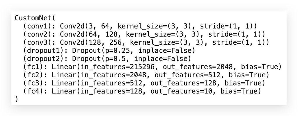
We now have the architecture we just created. This will be used to populate values within each component.
Our goal here is to learn the weights and coefficients. From there, we’ll be able to use the model to make predictions.
Let’s send the model to the device:
# 23. Define the device

# 23.a Check if a GPU is available; otherwise, use the CPU
device = torch.device("cuda:0" if torch.cuda.is_available() else "cpu")

# 23.b Print the selected device
print(device)

# -----> cuda:0
In our case, we’re using the GPU.
So, I’ll load the model into the GPU’s memory to speed up the process. Shortly, I’ll train the model directly on the GPU.
Here, we define the device, and then we send the model directly to the device:
# 23.c Send the model to the selected device
model.to(device)  # Moves the model to GPU if available; otherwise, keeps it on CPU
Done! The model is now on the device with its complete architecture.
The convolutional neural network architecture is finished. That’s it.
However, to make this work, I’ll need at least two more components.
17. Selecting the Loss Function
I want to explain the concept of the loss function in a very intuitive way and why we need it.
To do this, let’s do a mental exercise together. Follow along with me. I have the Forward method:
21.b Define the forward method for the forward pass
def forward(self, x):
This method is responsible for performing a training pass.
Let’s walk through a pass together. Imagine an image — a matrix of pixels.
 # 21.b.1 Apply the first convolutional layer
x = self.conv1(x)

# 21.b.2 Apply the ReLU activation function
x = F.relu(x)

# 21.b.3 Apply the second convolutional layer
x = self.conv2(x)

# 21.b.4 Apply the ReLU activation function
x = F.relu(x)

# 21.b.5 Apply the third convolutional layer
x = self.conv3(x)

# 21.b.6 Apply the ReLU activation function
x = F.relu(x)

# 21.b.7 Apply max pooling with a 2x2 kernel
x = F.max_pool2d(x, 2)

# 21.b.8 Apply the first dropout layer
x = self.dropout1(x)
I take this matrix and feed it into conv1. The conv1 layer applies a 3x3 kernel, multiplies it by the pixel matrix, and generates an output, which is the result of the mathematical operation.
Next, I pass this output through ReLU. If there’s a negative value, it becomes zero. If there’s a positive value, it remains in the resulting matrix.
I then take this resulting matrix and apply another convolutional layer. Once again, the kernel performs the multiplication.
I repeat this process, reducing the dimensionality step by step. Finally, I apply Dropout to prevent the model from learning the exact details of the pixels. What I want is mathematical generalization.
At this point, what we have is the learning of features or attributes, which are essentially the patterns within the pixels. This is what we have for the image.
Now, I need to classify what those pixels represent. To do that, I convert the matrix into a vector.
# 21.b.9 Flatten the tensor for the fully connected layer
x = torch.flatten(x, 1)
I then pass it through the fully connected layer.
# 21.b.10 Apply the first fully connected layer
x = self.fc1(x)
I apply ReLU.
# 21.b.11 Apply the ReLU activation function
 x = F.relu(x)
Exactly to include non-linearity, I apply Dropout to prevent the model from overfitting.
21.b.12 Apply the second dropout layer
x = self.dropout2(x)
I keep repeating the process, and when I reach Softmax, I’ll have class probability predictions.
So, for the image I started with, I’ll now have 10 predictions — 10 probabilities. I take the highest probability, which will be the predicted class.
Got it? That’s a full pass of an image — a matrix — through the entire architecture.
When it gets here:
# 21.b.18 Return the softmax output along dimension 1 (commonly used for classification)
return F.log_softmax(x, dim=1)
I now have the class prediction — the label prediction.
For that matrix, the prediction might indicate it’s a satellite image of an urban area, for example.
But did the model get the prediction right or wrong? Good question, isn’t it?
Is there any guarantee that the model will always predict correctly? Of course not. And at the beginning, it will make many more mistakes than correct predictions.
In other words, I need a way to measure whether the model is learning or not. That’s exactly the purpose of the loss function.
What does the loss function do? I feed the model with both input and output data, right?
So, I input the image, and for each image, I already know the output because I have the historical data.


I know the class — the label — of each image.
So, I feed the model with the input image, and it predicts the label. For example, imagine this first image. This first image is labeled as class 3, which represents Highway.
I gave the model the image of a highway. Instead of predicting it as a highway, the model predicted it as an industrial area. The model got it wrong, right?
Now, I’ll pass this result through the loss function.
Does the loss function know the true value? Yes, it does, because I have the historical data. This image should have been predicted as a highway. If the model predicted it as an industrial area, it made a mistake.
The loss function will calculate this error. That’s its purpose.
All of this boils down to a mathematical optimization problem. What we’re doing, essentially, is optimizing the loss function.
In other words, I want the smallest possible value for this function. The smallest value represents the smallest error, which is exactly what I want. I want the model to learn with the least possible error.
So, the entire learning process revolves around the loss function.
The loss function tells us when to stop training, whether the model is performing well, what strategies to use, and whether the architecture is appropriate. Without the loss function, how would I know if the model is learning or not?
The model makes a prediction. And now? Is the prediction correct or incorrect?
The loss function automates this process by comparing the model’s prediction to the true value. That’s why historical data is essential when training a model.
So, I’ve passed the data through the loss function. Excellent. I calculated the model’s error.
Now, imagine the error is high. What’s next? How do I tell the model:
“Hey, model, your error is too high. Learn the pixel details better.”
How do I tell the model it needs to learn in a better way?
That’s where the optimizer comes in.
18. Selecting the Optimizer
We have an architecture that allows the model to learn the organizational patterns of the pixels.
We also have the loss function, which helps us measure whether the model is learning or not.
But now, how do I tell the model:
“Hey, model, you made a mistake. Please improve in the next learning round.”
That’s the role of the optimizer.
The optimizer applies the backpropagation algorithm, which was actually developed in the 1980s. In fact, most elements of neural network architecture originated in the 1980s.
However, until around 2013, there weren’t enough images or computational power to make this work effectively. It was only after that point that things really took off, making these techniques incredibly effective today.
The backpropagation algorithm calculates the partial derivatives.
So, what does backpropagation do?
During training, what the neural network learns, in essence, is a set of numerical values. I know it’s hard to visualize this — I understand perfectly.
But try to make an effort right now. Look at these blocks of code here, these lines, and try to see them as just numbers.
# 21.b Define the forward method for the forward pass
    def forward(self, x):

        # 21.b.1 Apply the first convolutional layer
        x = self.conv1(x)

        # 21.b.2 Apply the ReLU activation function
        x = F.relu(x)

        # 21.b.3 Apply the second convolutional layer
        x = self.conv2(x)

        # 21.b.4 Apply the ReLU activation function
        x = F.relu(x)

        # 21.b.5 Apply the third convolutional layer
        x = self.conv3(x)

        # 21.b.6 Apply the ReLU activation function
        x = F.relu(x)

        # 21.b.7 Apply max pooling with a 2x2 kernel
        x = F.max_pool2d(x, 2)

        # 21.b.8 Apply the first dropout layer
        x = self.dropout1(x)

        # 21.b.9 Flatten the tensor for the fully connected layer
        x = torch.flatten(x, 1)

        # 21.b.10 Apply the first fully connected layer
        x = self.fc1(x)

        # 21.b.11 Apply the ReLU activation function
        x = F.relu(x)

        # 21.b.12 Apply the second dropout layer
        x = self.dropout2(x)

        # 21.b.13 Apply the second fully connected layer
        x = self.fc2(x)

        # 21.b.14 Apply the ReLU activation function
        x = F.relu(x)

        # 21.b.15 Apply the third fully connected layer
        x = self.fc3(x)

        # 21.b.16 Apply the ReLU activation function
        x = F.relu(x)

        # 21.b.17 Apply the fourth fully connected layer
        x = self.fc4(x)

        # 21.b.18 Return the softmax output along dimension 1 (commonly used for classification)
        return F.log_softmax(x, dim=1)
In practice, it’s all just numbers.
The model learns a set of weights and coefficients during training.
These weights are stored in the kernels used for convolution, max pooling, and the linear layers.
When the error is calculated, backpropagation computes the partial derivatives and updates the weights in the kernels and linear layers.
The model adjusts the weights, processes everything again, generates a new prediction, and the error is recalculated.
If the model improves, backpropagation continues adjusting the weights, step by step, during training.
All this happens in one line of code, using the ADAM optimizer:
# 25.a Define the optimizer as Adam
# Optimizer to adjust the model's weights
optimizer = optim.Adam(model.parameters())
This is one of the best optimization algorithms available for deep learning today.
The parameters shown here are the model parameters — the weights and coefficients. These are what will be updated during the next pass.
This architecture has three main components:
- The convolutional neural network, including the linear layer.
- The loss function.
- The optimization process with backpropagation.
The first component performs the forward pass — hence the forward method. The model makes a prediction, and the error is calculated.
Then comes the backward pass, or backpropagation, which updates the weights and coefficients in this cycle throughout the training process.
How long will this process last? That’s up to you. In our case, it will run for 30 epochs.
# 26.Define the number of training epochs
num_epochs = 30
This process will repeat for 30 epochs.
However, be careful. During each epoch, I’ll work with multiple batches of data. Since we have many images, I won’t load all of them into memory at once — it wouldn’t fit.
Instead, in one epoch, I’ll process the first batch, go through all the steps to generate the output, then process the second batch, and so on until all images are processed.
When the first epoch is complete, the model moves to the second. It takes what it has learned so far and continues.
For each batch, the calculations are done, the results are stored, and this flow continues until training is complete.
So, while it might seem like there are only 30 passes, each epoch consists of many batches worked on throughout the training process.
And this, essentially, is what people call artificial intelligence, which, as you might agree, has no intelligence at all.
If there’s any intelligence, it lies in the person sitting at the computer building all this. The model itself is just performing mathematical calculations at high speed.
Now, let’s execute and create the loss function:
# 24. Loss function - Define the loss function as Cross Entropy Loss
criterion = nn.CrossEntropyLoss()
Now, let’s execute and create the optimizer:
# 25. Define the optimizer as Adam - Optimizer to adjust the model's weights
optimizer = optim.Adam(model.parameters())
Now, let’s prepare the training loop.
We’ll bring everything together: the deep learning architecture and the data.
19. Building the Training Loop
Let’s build the training loop.
First, I’ll define the number of epochs, essentially the time we’ll have to train the model.
# 26.Define the number of training epochs
num_epochs = 30
There are several strategies here.
One approach is to set a fixed number of epochs — train for 30 epochs, or any number you choose, like 50, 60, or 70.
Another approach is to use callbacks. For example, you define a larger number of epochs, such as 100, and monitor the training.
If the model stops improving for 5 consecutive epochs, you end the training. This is useful for avoiding overfitting and is a valid strategy.
A third approach, also using callbacks, is to monitor the training and, if learning stalls — meaning the model’s performance isn’t improving based on the metrics — you give it a little boost by adjusting the learning rate. Yes, you give it a “push.”
The human plays an active role in this entire process. You’re the one responsible for defining how the training process will proceed.
In this case, I’ll train for 30 epochs. Here’s the testing iteration:
# 27. Test iteration - Initializes an iterator to sample data from the testing set
test_iter = iter(testing_dataloader)
And here is the training loop:
%%time
print('Training Started!')

# 28. Iterate through the number of epochs
for epoch in range(num_epochs):

    # 28.a Initialize the variable to accumulate loss over the epoch
    running_loss = 0.0

    # 28.b Initialize a counter for the batches
    i = 0

    # 28.c Iterate over the training data with a progress bar (tqdm)
    for data in (pbar := tqdm(training_dataloader)):

        # 28.c.1 Update the progress bar description to show the current epoch
        pbar.set_description(f"\nEpoch {epoch}")

        # 28.c.2 Unpack the batch data into inputs and labels
        inputs, labels = data

        # 28.c.3 Move inputs and labels to the appropriate device (CPU or GPU)
        inputs, labels = inputs.to(device), labels.to(device)

        # 28.c.4 Zero the gradients of the optimizer
        optimizer.zero_grad()

        # 28.c.5 Perform the forward pass through the neural network
        outputs = model(inputs)

        # 28.c.6 Calculate the loss using the defined criterion
        loss = criterion(outputs, labels)

        # 28.c.7 Perform the backward pass to calculate gradients
        loss.backward()

        # 28.c.8 Update the neural network weights using the optimizer
        optimizer.step()

        # 28.c.9 Update the accumulated loss value
        running_loss += loss.item()

        # 28.c.10 Initialize counters for the number of correct predictions and total samples
        total_correct = 0
        total_samples = 0

        # 28.c.11 Perform validation every 100 batches
        if i % 100 == 0:

            # 28.c.11.a Disable gradient computation to save memory and processing time
            with torch.no_grad():

                # 28.c.11.b Get a batch of test images and labels
                test_images, test_labels = next(test_iter)
                test_images, test_labels = test_images.to(device), test_labels.to(device)

                # 28.c.11.c Perform a forward pass on the neural network with 8 test images
                test_outputs = model(test_images[:8])

                # 28.c.11.d Get predictions for the 8 test images
                _, predicted = torch.max(test_outputs, 1)

        # 28.c.12 Increment the batch counter
        i += 1

    # 28.d Display the average loss for the epoch
    print(f"Epoch {epoch}, Loss: {running_loss / (i)}")

print('Training Completed!')
The training loop begins with a for loop iterating through 30 epochs.
At the start of each epoch, the model’s error is reset, and a specific counter is initialized to track batches.
Data is fetched from the training_dataloader, and a progress bar (pbar) is used, courtesy of the tqdm package. While optional, this progress bar visually indicates that training is underway, which is especially helpful for longer processes.
Next, the input data and labels are moved to the device (GPU memory), along with the model itself, to minimize the latency caused by communication between the CPU and GPU.
The optimizer’s gradients are reset at the start of every batch. Then, a forward pass is performed: inputs are fed into the model, and predictions are generated.
The predictions are compared with the true values using the loss function, resulting in an error calculation.
This error is passed through backpropagation, which computes the gradients. The optimizer then updates the model’s weights, ensuring it continues to learn during the next pass.
Throughout this process, the accumulated error is tracked, and the batch counter is incremented. For every 100 batches, a progress message is printed to provide feedback on the training status.
This approach balances clarity and avoids excessive output, which could clutter the logs or impact performance.
At the end of each epoch, the current error and epoch number are displayed. The loop continues until all epochs are completed. This, in essence, is the training loop.
20. Model Training
Notice that for each epoch, we have a progress bar reflecting the batches of data being processed, right?
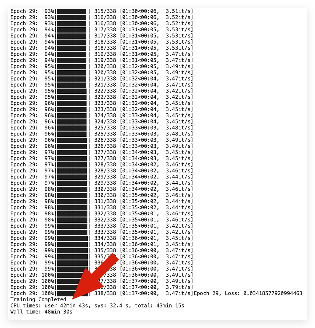
These numbers change because I’m working with multiple batches — new images from the training dataset are fed into the model during training.
What’s happening here? It’s the entire process I explained earlier.
The model receives the batches of images, processes them using the forward method, makes predictions, calculates the error, applies backpropagation, updates the weights for the next pass, and continues learning.
At the end, we calculate the metrics and evaluate the model.
Using our resources in Colab, with the dataset, Python code, and this setup, we’re building something resembling “intelligence.” Essentially, it’s learning through our beloved mathematics.
The model is learning the patterns in the data, and as a result, we’ll have a model capable of classifying images.
This type of technology is increasingly used today — facial recognition, drone-based recognition, medical image analysis — virtually any domain involving images or videos can leverage this strategy.
The most advanced architectures today in computer vision use some form of convolutional neural networks (CNNs).
There hasn’t been a much better learning strategy for images than convolution.
Convolution remains the cornerstone of these architectures. While we can combine different alternatives and architectures, convolution is still the best strategy.
21. Model Evaluation
The free version of Colab, with its 15 GB of GPU memory, allows you to train this model without any issues.
Notice that we’ve reached the final stage, with this model error rate.

Notice that the epoch is 29. Why is that? If I set 30 epochs, you already know — it’s because indexing in Python starts at 0.
So, we have epochs ranging from 0 to 29, totaling 30 epochs. Exactly.
And the error is 0.034, which means the smaller the error, the better. The error seems very low, but let’s evaluate the model to verify if it truly has good performance.
Let’s go ahead and define the counters:
# 29. Initialize counters

# 29.a Counter for the number of correct predictions
total_correct = 0  # Tracks the total number of correct classifications

# 29.b Counter for the total number of samples
total_samples = 0  # Tracks the total number of samples evaluated
Then, we need to set the model to evaluation mode. This is required in PyTorch.
I’ll do this by calling model.eval():
# 30. Evaluate the model

# 30.a Set the model to evaluation mode (disables layers like dropout and batch normalization)
model.eval()

# 30.b Disable gradient calculation to save memory and processing time
with torch.no_grad():

    # 30.c Iterate over the testing data with a progress bar (tqdm)
    for data in (pbar := tqdm(testing_dataloader)):

        # 30.c.1 Update the progress bar description to show "Evaluating Model"
        pbar.set_description(f"Evaluating the Model.")

        # 30.c.2 Unpack the batch data into inputs and labels
        inputs, labels = data

        # 30.c.3 Move inputs and labels to the appropriate device (CPU or GPU)
        inputs, labels = inputs.to(device), labels.to(device)

        # 30.c.4 Perform the forward pass through the model
        outputs = model(inputs)

        # 30.c.5 Get the predicted class (index of the maximum value) for each input in the batch
        _, predicted = torch.max(outputs.data, 1)

        # 30.c.6 Increment the total number of samples by the batch size
        total_samples += labels.size(0)

        # 30.c.7 Increment the total number of correct predictions for the current batch
        total_correct += (predicted == labels).sum().item()

Next, I’ll specify the following: no weight updates and no gradient updates are needed.
Since the model is in evaluation mode, I only want to execute the architecture to obtain the model’s predictions. Gradients — partial derivatives — are only updated during training. Afterward, there’s no need for that, which is why we set the model to eval mode.
Then, I fetch the data from the testing_dataloader, prepare the description, and extract the data.
The data is sent to the device (e.g., GPU), and predictions are made using the model.
To process the output, I use torch.max. When the model delivers predictions, it provides 10 predictions for each image.
Why 10 predictions? Because we have 10 classes. Each prediction represents the probability of a class.
However, I don’t want all 10 predictions. If needed, I could extract and use them, but my focus is the final class prediction.
To achieve that, I’ll take the highest value using torch.max, which represents the highest probability, and assign that as the predicted class.
Now, let’s calculate the model’s accuracy:
# 31. Calculate accuracy

# 31.a Compute the accuracy as the ratio of correct predictions to total samples
accuracy = total_correct / total_samples

# 31.b Print the calculated accuracy
print(accuracy)  # Displays the overall accuracy of the model

# -----> 0.8177777777777778
For every 100 predictions, the model gets 81 correct. That’s excellent performance, especially considering this is the first version of the model.
You can always go back and optimize the hyperparameters, modify the architecture, train for a longer time, or adjust the batch size. There are many possibilities to further improve this performance.
For our example, however, this is more than sufficient.
Now, let’s deploy and use the model.
22. Deploying and Using the Model
We can now deploy the model to make predictions.
It will generate the image along with the predicted class.
Here we have the satellite image and the model’s prediction, considering its accuracy level of 81%.
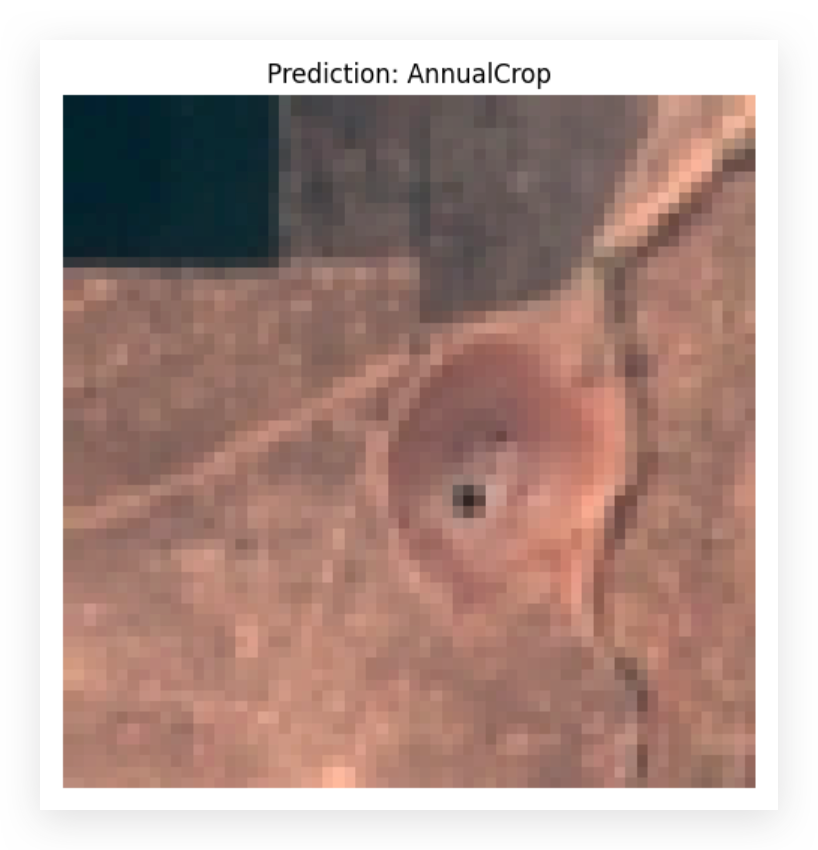
Each time you execute the notebook, the image will be different.
I’m fetching the image randomly. If you run it again, the prediction loop with the model deployment will execute once more, providing a new image and prediction.
# 32. Evaluate and use the model for prediction

# 32.a Set the model to evaluation mode
with torch.no_grad():

    # 32.a.1 Get the first batch of data
    data_iter = iter(testing_dataloader)
    data = next(data_iter)

    # 32.a.2 Extract the inputs (images) from the batch
    inputs, _ = data

    # 32.a.3 Select the first image from the batch
    image = inputs[0].unsqueeze(0)

    # 32.a.4 Move the image to the same device as the model
    image = image.to(device)

    # 32.a.5 Perform inference to get the model's prediction for the image
    outputs = model(image)

    # 32.a.6 Get the index of the predicted class
    _, predicted = torch.max(outputs, 1)

    # 32.a.7 Convert the image to a NumPy array for visualization
    image_numpy = image.cpu().numpy()[0]  # Move the image back to CPU and convert to NumPy

    # 32.a.8 Rearrange dimensions from [C, H, W] to [H, W, C] for visualization
    image_numpy = np.transpose(image_numpy, (1, 2, 0))

    # 32.a.9 Adjust image channels if necessary
    if image_numpy.shape[2] == 1:  # Grayscale images
        image_numpy = np.squeeze(image_numpy, axis=2)
    elif image_numpy.shape[2] == 3:  # RGB images
        # Normalize to the range [0, 1] for proper visualization
        image_numpy = (image_numpy - image_numpy.min()) / (image_numpy.max() - image_numpy.min())

    # 32.a.10 Display the image with its predicted label
    plt.figure(figsize=(6, 6))
    plt.imshow(image_numpy)
    plt.title(f'Prediction: {class_mapping[predicted.item()]}')
    plt.axis('off')
    plt.show()
Wait a few moments, and another image will be displayed for you.
Notice that it’s a different image with the model’s prediction. This process continues. Each time you execute the notebook, you’ll get a new prediction.
So, what do we have in the loop? Not much else is needed.
First, I’ll set the model to evaluation mode again. This ensures no gradient calculations, as the model is now being used for predictions.
Next, I’ll fetch data from our testing_dataloader. Alternatively, we could create a different dataloader with other images.
Once the inputs are obtained, an underscore appears here:
# 32.a.2 Extract the inputs (images) from the batch
    inputs, _ = data
23. Finalizing the Model
What is this underscore here? What’s it doing? It’s not misplaced — it serves a very important role.
When fetching data earlier for evaluation, I retrieved both inputs and labels to evaluate the model. Now, I don’t need the labels; I’m satisfied with the performance. At this point, I only want to use the model.
Thus, I discard the labels using the underscore (_). This is a programming strategy.
Next, I’ll select the first image from the batch returned by the dataloader, move it to the device (GPU), and make a prediction with the model.
What does the model output? It gives ten probabilities — one for each class. I take the highest probability and set it as the predicted class.
The image is then moved to the CPU and converted to a NumPy format for visualization. The pixel matrix is transformed into an image format so we can view it. The channels are transposed and adjusted, normalized, and finally printed along with the predicted class.
This cell can be executed as many times as you like. It will fetch a new image each time from the test dataloader, make a prediction, and display the result. If you wanted to use a completely different image, you could load it separately and predict its class.
Now, an interesting question arises: What if I provide an image of a cat to the model?
The model will still output a class prediction. That’s the problem — it doesn’t know what a cat is. The model will process the cat image as a pixel matrix and look for patterns it has learned. It might mistakenly predict the cat as a river, for instance, if the pixel patterns resemble those of a river class.
This highlights an important concept: the model can only predict based on the ten classes it was trained on.
If you want the model to recognize cats, you’ll need to:
- Gather thousands of cat images.
- Add them to the dataset.
- Introduce a new class, “cat.”
- Retrain the model.
The same applies if you want the model to predict dogs or even 500 different classes. You need to provide images for all 500 classes, train the model, and it will then be capable of making predictions for those classes.
This demonstrates that a model isn’t fully automatic — it’s limited to what it has been trained on. To make it predict more, you have to teach it more.
Is this concept clear?
We’ve trained this satellite image classification model in just 40 minutes, producing a solution that’s capable, efficient, and cost-effective.
Does this solve the company’s problem? If yes, the project is complete, the client is happy, and we can move on to the next project.
Thank you for following along! 🐼❤️
All images, content, and text by Leo Anello.
Bibliography, References, and Useful Links
Project Repository on GitHub
PyTorch documentation - PyTorch 2.5 documentation
torchvision - Torchvision 0.20 documentation
Satellite Image Classification Using Deep Learning | By Leo Anello | Medium was originally published in Towards Data Science on Medium, where people are continuing the conversation by highlighting and responding to this story.
from Datascience in Towards Data Science on Medium https://ift.tt/l9DuPe4
via IFTTT


