Sentiment Analysis with Transformers: A Complete Deep Learning Project — PT. II
Sentiment Analysis with Transformers: A Complete Deep Learning Project — PT. II
Master fine-tuning Transformers, comparing deep learning architectures, and deploying sentiment analysis models

1. Continuing…
Now, I’ll bring you part 2 of the project. This project began in the previous tutorial. The proposal of this project is to build three versions of a deep learning model.
A simpler version, which we created in the previous tutorial:
Sentiment Analysis with Transformers: A Complete Deep Learning Project — PT. I
An intermediate version, and finally, the most advanced version with today’s state-of-the-art in artificial intelligence, which is the Transformer model. Then, we will proceed with FineTuning. With this project, you will now have a benchmark for comparison.
By the end of this tutorial, I will even conduct a comparison round. I will compare the architectures we created and the complexity of building each model.
I will compare the evaluation of each model. Finally, I will compare the deployment process. At the end of this project, you will have a very clear view of what deep learning is, across three different levels.
With a simpler architecture, an intermediate one, and a more advanced one. Concluding the project, you will be ready to follow increasingly advanced projects I might eventually bring here. Let’s raise the bar.
At the end of the article, don’t forget to leave your claps generously. The link to my GitHub with the complete and impeccable project notebook will be available at the end of the tutorial for you to use. Let’s get started!
2. Hardware Recommendation
In the previous tutorial, we trained version 1 of the model. Now, we will train versions 2 and 3. These two versions are significantly heavier, especially version 3. It’s important to discuss hardware recommendations at this stage.
I’ve already run this part of the project on various machines and in cloud environments to get an accurate idea of execution times and provide them as a reference for you. I used version 3 as the baseline for these tests.
Version 2 isn’t as heavy. While heavier than version 1, it remains manageable. Version 3, however, is much heavier and requires better hardware. I started by testing without a GPU and then with one.
On a machine with a Core i7 processor (my desktop), training version 3 took 1 hour and 25 minutes — almost an hour and a half. Then, I tested on another machine, an Apple M2, which is simply phenomenal, and the training time dropped to 32 minutes. This was without a GPU, just to clarify.
As expected, using a GPU significantly improved performance. The model is heavy, and parallelizing operations with a GPU dramatically reduces training time. Using the free tier of Colab with a T4 GPU, the training time dropped to 8 minutes.
If you have a machine with a GPU or a Colab subscription, I encourage you to experiment. This will significantly accelerate training time. Therefore, I recommend you execute part 2 of the project with me on Google Colab.
3. Reviewing Part 1
I’ll start by reviewing and executing part 1 of this project, which we worked on in the previous tutorial. The first step is to install the necessary packages.
You’ll execute each of the initial cells. These are essentially the same packages we used in the previous tutorial. For example, the Watermark package is used to generate a watermark:
!pip install -q -U watermark
For text data processing, we’ll use Spacy:
!pip install -q spacy
We’ll use TensorFlow to train the model.
!pip install -q tensorflow
For version 3 of the project, we’ll use the Transformers library.
!pip install -q transformers
Below, I’m disabling any type of warning or information from TensorFlow. I want log level 3 — errors only.
If there’s an error, show it. If not, there’s no need to display anything:
%env TF_CPP_MIN_LOG_LEVEL=3
Next, we load the packages into the session:
# 1. Imports
import math
import nltk
import spacy
import numpy as np
import pandas as pd
import tensorflow as tf
import matplotlib.pyplot as plt
import transformers
from tokenizers import BertWordPieceTokenizer
from tqdm import tqdm
from nltk.corpus import stopwords
from sklearn.preprocessing import LabelEncoder
from sklearn.feature_extraction.text import TfidfVectorizer
from sklearn.model_selection import train_test_split
from sklearn.utils.class_weight import compute_class_weight
from sklearn.metrics import confusion_matrix, accuracy_score, classification_report
from tensorflow.keras.utils import to_categorical
from tensorflow.keras.models import Sequential
from tensorflow.keras.models import load_model
from keras_preprocessing.text import Tokenizer
from keras_preprocessing.sequence import pad_sequences
from keras.metrics import Precision, Recall, AUC
from keras.layers import Embedding, LSTM, Dense, Dropout, Bidirectional
from keras.callbacks import EarlyStopping, LearningRateScheduler, CallbackList, ReduceLROnPlateau
from tensorflow.keras.optimizers import Adam
from tensorflow.keras.regularizers import l1_l2
from keras.saving import register_keras_serializable
from tensorflow.keras.layers import Layer, Dense
from transformers import TFDistilBertModel, DistilBertConfig
from tensorflow.keras.metrics import Precision, Recall, AUC
import warnings
warnings.filterwarnings('ignore')
Basically, the same packages we used before. At the end of the imports, I’m just silencing any type of warning to avoid cluttering the notebook.
After that, you enable the Watermark package:
%reload_ext watermark
%watermark -a "Your_Name"
I will then load the data, starting with the training data, followed by the test data:
# 2. Loading Training Data
training_data = pd.read_csv('training_data.txt', header=None, delimiter=';')

# 2. Loading Test Data
test_data = pd.read_csv('test_data.txt', header=None, delimiter=';')
Next, adjust the column names:
# 3. Adjusting Column Names
training_data = training_data.rename(columns={0: 'text', 1: 'sentiment'})
test_data = test_data.rename(columns={0: 'text', 1: 'sentiment'})
All of this was done in the previous tutorial, which is why I’m not diving too deep into it, ok?
We then check the shape of both the training and test datasets:
# 4. Checking Dataset Shape
training_data.shape

# -----> (16000, 2)

# 5. Checking Test Dataset Shape
test_data.shape

# -----> (2000, 2)
We verify a sample of the data using our default approach:
# 6. Training Data Sample
training_data.head()
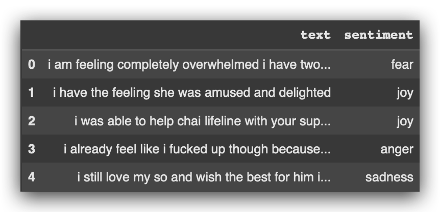
After that, I’ll return the count of elements for each category, for each sentiment, in both the training and test datasets:
# 7. Sentiments in Training Data
training_data['sentiment'].value_counts()

# 8. Sentiments in Test Data
test_data['sentiment'].value_counts()
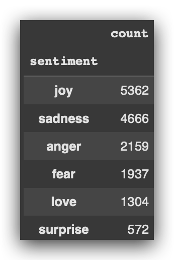
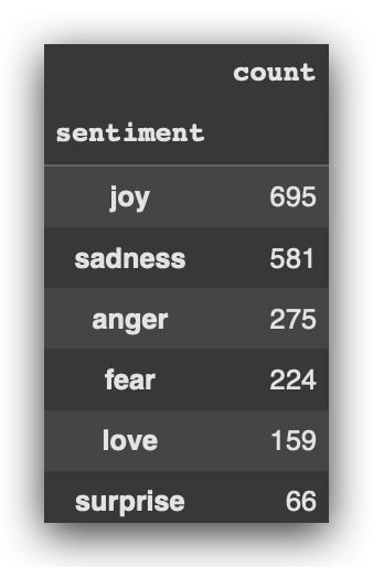
We will then preprocess the data using Spacy. Here’s an important point: I’ll also use this preprocessing with Spacy for versions 2 and 3.
The data preprocessing done with Spacy will be the same for versions 1, 2, and 3, ensuring a fair comparison of the model versions.
First, let’s install and download the dictionary:
!python -m spacy download en_core_web_md -q

After that, load the dictionary:
# 9. Load SpaCy Model
nlp = spacy.load('en_core_web_md')
We then create the function to process the text:
# 10. Definition of the 'preprocess_text' Function, Which Takes a Text as a Parameter
def preprocess_text(text):

    # 10.a Process the text using the SpaCy model
    doc = nlp(text)

    # 10.b Create a list of lemmatized tokens, converted to lowercase, stripped of whitespace,
    # excluding stopwords
    tokens = [token.lemma_.lower().strip() for token in doc if not token.is_stop]

    # 10.c Return the processed tokens as a single string, joined with spaces
    return ' '.join(tokens)
I then apply the function to both the training and test datasets:
# 11. Apply the Preprocessing Function to Training Data
training_data['processed_text'] = training_data['text'].apply(preprocess_text)

# 12. Apply the Preprocessing Function to Test Data
test_data['processed_text'] = test_data['text'].apply(preprocess_text)
Next, I check a sample of the data:
# 13. Data Sample
training_data.head()

All of this is done so we can perform lemmatization, which replaces some words with their root forms. This simplifies the text data, enabling us to train the deeplearning models more effectively.
I’ll execute all the cells from version 1 up to the point where version 2 starts, at command #57.
Keep scrolling and executing, and I’ll do the same from here.
4. Model V2 — LSTM (Long Short-Term Memory)
Now we will create the second version of the model, using a different architecture: LSTM. In version 2, we’ll work with a more robust architecture compared to the fully connected architecture from version 1.
The LSTM is excellent for tasks in Natural Language Processing. It also performs well with time series data, as it works with sequential inputs. These sequences can be text data (sentences) or, for example, time series data.
However, LSTM has a significant limitation: it struggles with long-term context. During training, it loses information over the long term due to the vanishing gradient problem. As the gradient diminishes, it eventually disappears, limiting its capacity for larger datasets or extended contexts.
If the goal is for the model to learn something extensive, such as the entire content of a book, LSTM won’t suffice. For that, you need the Transformer, which we’ll explore in version 3 shortly.
To construct the LSTM, I’ll use the data I prepared with Spacy. The vectorization preparation done for version 1 is no longer relevant here. From this point forward, I’ll use the data processed with Spacy.
# 11. Apply the Preprocessing Function to Training Data
training_data['processed_text'] = training_data['text'].apply(preprocess_text)

# 12. Apply the Preprocessing Function to Test Data
test_data['processed_text'] = test_data['text'].apply(preprocess_text)
Then, I’ll prepare the data for LSTM. Later, I’ll do the same for version 3, where I’ll use the BERT model, a Transformer model.
This approach provides an important first comparison. Starting with the same dataset, already processed with Spacy, I’ll need to make different transformations according to the architecture.
Many people often place excessive emphasis on the model architecture and overlook the importance of data. In other words, three different models will require three distinct data preprocessing steps.
5. Model V2 — Tokenization and Padding
Our first task in version 2 is to prepare the tokenization. We’ll use the same processed data we prepared with Spacy. In other words, for version 2, I’ll use the same data used in version 1.
Now, I’ll proceed with the specific preparation for version 2. Next, I’ll load the tokenizer, which in this case will be our tokenizer:
# 58. Create the Tokenizer
# from keras.preprocessing.text import Tokenizer
tokenizer = Tokenizer()
What is tokenization? It’s the process of splitting text data into smaller portions. In this case, since I’m not customizing anything, I’ll split sentences into words.
However, a token — the smallest unit — could also be an entire sentence. Some modern AI models use sentences as tokens, resulting in high-precision models for Natural Language Processing (NLP).
Here, I’ll work with tokenization at the word level, splitting sentences into words. I’ll create the tokenizer and call it tokenizer. Next, I’ll train this tokenizer on the training data:
# 59. Fit the Tokenizer with Processed Texts
tokenizer.fit_on_texts(training_data['processed_text'])
What exactly is the tokenizer being trained on? It will identify the tokens based on our dataset. From this, it will generate the final words from each word and then create an index. Once that’s done, the tokenizer is built.
Next, we’ll extract the word index from the tokenizer and store it in a Python variable, word_index:
# 60. Extract Word Index
word_index = tokenizer.word_index
Let’s check the length:
# 61. Check the Length of the Word Index
len(word_index)

# -----> 11897
The 11897 is the total index length.
I’ll print a few lines of this index for you:
# 62. Iterate Over Key-Value Pairs in the Dictionary
for i, (key, value) in enumerate(word_index.items()):
    print(key, value)
    # Break the loop after printing 10 items
    if i == 9:
        break

# ------>
'''
feel 1
like 2
m 3
not 4
feeling 5
know 6
time 7
t 8
want 9
think 10
'''
What does this look like to you? I have a word and a number. So, it’s an index — a classic mapping. Each word from our training dataset has now been assigned an index.
We have the processed text data, and the tokenizer split each sentence into words and assigned an index to each word. This is exactly what we see above. I’m only printing the first 10 entries, but the index contains 11,897 items.
Next, I’ll take the text dataset and replace the words with their respective codes, or numbers. As you know, we cannot train the model with text data. Training requires numerical values.
However, this conversion to numeric values cannot be done randomly. That’s why I’m creating an index using tokenization. Shortly, I’ll use this tokenizer to replace all the words in the data with their corresponding codes.
This approach works well but has a limitation: it doesn’t effectively capture the context. It maps each word and its order but struggles with broader context. To handle that, we’d need a different tokenization strategy, like the one we’ll use with the Transformers in version 3.
In Transformers, we do something similar, but the indices also incorporate context. With LSTM, it’s essentially a simple mapping: each word gets a code.
Now, I’ll take the tokenizer, which already has this index, and use the function texts_to_sequences:
# 63. Convert Training Texts to Token Sequences
train_sequences = tokenizer.texts_to_sequences(training_data['processed_text'])
What does it do? It takes our dataset and replaces each word with its corresponding code, creating a large numeric matrix.
# 64. Define the Maximum Length of Sequences
max_length = 100
I’ll work with a maximum length of 100. What does this mean? Each sentence will have, at most, 100 positions. I won’t work with sentences longer than that.
You’d agree that sentences will have varying lengths, right? So, I’m telling the model that I know the sentences aren’t the same size. I’ll adjust them to all have the same size — up to 100 positions.
But this introduces a problem. If I limit them to 100 positions, and their lengths vary, how do I make them the same size? Models operate exclusively with matrices, so I need matrices with uniform proportions.
If I feed text data with sentences of varying sizes, training the model won’t work because matrix operations require consistency.
How do we solve this? It’s simple — this is where the idea of padding comes in.
# 65. Padding Training Sequences
train_sequences_padded = pad_sequences(
train_sequences, maxlen=max_length, truncating='post')
What does padding do? It takes each sentence and fills it — usually with zeros or another character — up to 100 positions.
Looking at the data, you’ll notice, for example, that the second sentence is shorter and has empty spaces.

What does it do here? It fills sentences with a character, usually the digit zero. That’s it. If a sentence has fewer than 100 positions, it fills it until it reaches 100.
But what if a sentence has more than 100 positions? That’s where truncating='post' comes in. This ensures truncation happens at the end of the text.
This is all explained in the notebook, so feel free to read it for additional details. Essentially, I’ll take the training sequences and apply padding. This ensures everything has a length of up to 100.
If a sentence exceeds 100 positions, the extra positions will be truncated from the end. Yes, that’s the trade-off. If you don’t want to lose any part of the text, you’ll need to increase the maximum length.
However, increasing the length will also increase the size of the matrix, leading to longer training times. If you want to avoid truncation, simply increase the length here:
# 64. Define the Maximum Length of Sequences
max_length = 100
The matrix will become larger, and it will take more time to train the model. Feel free to experiment with this. Try other options later and evaluate the results.
We’ve now completed tokenization and padding for the training data. Let’s proceed to apply tokenization and padding to the test data:
# 66. Convert Test Texts to Token Sequences
test_sequences = tokenizer.texts_to_sequences(test_data['processed_text'])
Next, we also apply padding to the test data:
# 67. Padding Test Sequences
test_sequences_padded = pad_sequences(test_sequences, maxlen=max_length)
At this point, we have matrices with input data already in numeric format. What preprocessing have we done so far? Tokenization and padding.
In version 1, we used TF-IDF, another strategy to convert text into numbers. The choice of text processing strategy is up to you. I’ve opted to showcase different strategies for two reasons:
- To teach you new strategies: In version 1, I used TF-IDF, and now I’m using tokenization. The goal remains the same: to convert text into numerical representation. This way, you get to learn multiple approaches.
- Because tokenization is the modern standard: Today, most transformers, LLMs, and state-of-the-art AI models rely heavily on tokenization. While TF-IDF is good to know and can be used in specific cases, tokenization is the preferred method.
Remember, you don’t always need to use a cannon to kill a mosquito. TF-IDF is a valid technique, but modern approaches lean towards tokenization. That’s why I’m using it in version 2 and will also use it in version 3.
For more advanced AI models, like BERT—an LLM I’ll introduce soon—we typically use tokenization, which also incorporates context. The tokenization done here doesn’t include context because LSTM cannot effectively handle it; it loses context over time.
It wouldn’t make sense to attempt contextual tokenization here. Instead, we’re using what LSTM can process. As the data becomes increasingly complex, working with context becomes more relevant. That’s why I’ll use another type of tokenization in version 3.
The input data is now ready. Let’s prepare the output data next.
6. Model V2 — Encoding the Target Variable
We’ve already processed the input data. What are the input data in our case? The processed_text column:

At this point, we already have the matrix, and it has uniform dimensions because we applied padding. Soon, we’ll convert this matrix into an embedding, which is the gateway for training the model.
Now, I need to prepare the output data, which is the target variable, sentiment. Currently, it’s in text format, right? That won’t work, because everything boils down to mathematics. I need to convert it into a numeric representation.
For this, I’ll use the same strategy as in version 1: label encoding. Let’s create the LabelEncoder:
# 68. Create the Label Encoder
label_encoder_v2 = LabelEncoder()
In this case, I’ve named it label_encoder_v2. I’ll then apply fit_transform to the training data:
# 69. Fit and Transform Sentiment Labels for Training
y_train_le = label_encoder_v2.fit_transform(training_data['sentiment'])
Let’s prepare y_train_le:
# 69. Fit and Transform Sentiment Labels for Training
y_train_le = label_encoder_v2.fit_transform(training_data['sentiment'])
And I’ll simply apply transform to the test data:
# 70. Transform Sentiment Labels for Testing
y_test_le = label_encoder_v2.transform(test_data['sentiment'])
Which is similar to what we did in version 1.
I’ll now adjust the labels to categorical variables:
# 71. Convert Labels to Categorical Variables
y_train_encoded = to_categorical(y_train_le)
y_test_encoded = to_categorical(y_test_le)
I’ve already processed the output data. The output data is now in numeric representation, with each sentiment assigned a number.
At this point, I have the input matrix, where each word in each sentence is represented by a number. I also have the output variable, where each sentiment is also represented by a number.
Whenever we work with NLP (Natural Language Processing), this step is essential. The technique, strategy, or approach may vary, but this process remains constant.
You take your text data and apply some strategy to convert it into numbers. In version 1, I introduced TF-IDF. Now, in version 2, I’m using direct tokenization.
Let’s define the vocabulary size and proceed to build the architecture for version 2 of our model.
7. Model V2 — Vocab Size & Embedding Dimension
The next step is to define the vocabulary size and the embedding dimension.
What does this mean? Notice that I have the tokenizer and the word_index here:
# 72. Define Vocabulary Size
vocab_size = len(tokenizer.word_index) + 1
What is this word index? It’s essentially a dictionary.
Each word is associated with a number. And where do these words come from? From our dataset, right? That’s where I applied the tokenizer.
This is the vocabulary size stored in the vocab_size object. I’m adding one at the end because Python indexing starts at zero. Let’s take a look:
# 73. Print Vocabulary Size
print(vocab_size)

# -----> 11898
Here is the vocabulary size. What does this mean in practice? This is NLP (Natural Language Processing).
In this case, I have the processed_text column:

I have numerous sentences in the dataset. We applied the tokenizer, and each sentence received a number. This determines the size of the vocabulary.
The model will only be capable of making predictions with words that exist within this vocabulary. Anything outside the vocabulary will be beyond the model’s ability to handle.
This is similar to making predictions for predefined classes. For example, in the case of sentiment analysis, we have six sentiments in the dataset, right?
The model won’t be able to predict a seventh sentiment because it wasn’t trained to do so. It only learned about six sentiments, and that’s all it can predict.
The same principle applies to the vocabulary. The model’s performance is restricted to the vocabulary size, which essentially reflects the dataset used for training.
If you want a model capable of predicting anything for any text data, is it possible? Sure, it is! You’d need to create a massive vocabulary. However, this would require terabytes of storage and significant computational capacity.
Our model now has this vocabulary. These are the words it will use for training. It will learn within this context and limitation, which is essentially what we refer to in machine learning as the hypothesis space.
The model won’t perform anything outside this space. If you want to expand this space, you can bring in more text data, increasing the vocabulary size — though this will have an impact on resource requirements.
# 74. Define Embedding Dimension
embedding_dim = max_length
Next, I define the size of the embedding, which is essentially the data matrix we’ll use to feed the model:
8. Model V2 — Model Construction
We can finally build our model.
Often, we don’t give enough importance to the process, but getting to this point is a journey — it involves careful data preparation, which cannot be skipped.
Let’s set up a sequence of layers using Keras, which is now part of TensorFlow:
# 75. Construct the LSTM Model
model_v2 = tf.keras.Sequential([

    # 75.a Embedding layer with the vocabulary size, embedding dimension, and input length
    Embedding(vocab_size, embedding_dim, input_length=max_length),

    # 75.b Bidirectional LSTM layer with 64 units
    Bidirectional(LSTM(64)),

    # 75.c Dropout layer to prevent overfitting
    Dropout(0.4),

    # 75.d Dense layer with 32 units, Leaky ReLU activation, and L1/L2 regularization
    Dense(32, activation='leaky_relu', kernel_regularizer=l1_l2(l1=0.01, l2=0.01)),

    # 75.e Additional Dropout layer
    Dropout(0.4),

    # 75.f Output layer with 6 units and softmax activation for multi-class classification
    Dense(6, activation='softmax')
])
I’ll use the Embedding layer to create the input matrix with dimensions (vocab_size, embedding_dim).
The input length will be input_length=max_length, which is set to 100.
I won’t process anything beyond this length. If you want to increase it, you can simply adjust the max_length parameter.
I’ll also include a Bidirectional layer, which is standard for LSTM.
This layer encapsulates the structure of a recurrent neural network, incorporating the concept of gates that gradually allow predictions as training progresses.
For the LSTM, I’ll use 60 neurons. This is a configurable parameter. After that, I’ll apply a dropout layer for regularization.
Dropout helps discard some results during training to prevent overfitting, as LSTM models tend to have high learning capacity.
If the model learns too much, it risks capturing unnecessary details from the data, which we want to avoid. Our goal is a generalizable model. Dropout helps achieve this.
Next, within the same block, I’ll include a dense layer:
# 75.d Dense layer with 32 units, Leaky ReLU activation, and L1/L2 regularization
    Dense(32, activation='leaky_relu', kernel_regularizer=l1_l2(l1=0.01, l2=0.01)),
Look how cool this is — dense layer. This is essentially the structure of the model we created in version 1.
Let’s revisit the architecture. Didn’t we create dense layers there as well?
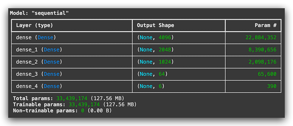
This was version 1, right? In other words, I only used this type of layer. However, the dense layer is generally used at the very end of almost any Deep Learning architecture.
Why is that? Because this layer allows for the learning of all the outputs from all the mathematical neurons.
So, in version 1, I exclusively used the dense layer. Now, in version 2, I’m using an LSTM layer combined with a dense layer at the very end:
 # 75.d Dense layer with 32 units, Leaky ReLU activation, and L1/L2 regularization
  Dense(32, activation='leaky_relu', kernel_regularizer=l1_l2(l1=0.01, l2=0.01)),
In this configuration, I’m using a leaky_relu activation function in the dense layer, combined with L1 and L2 regularization.
This is to prevent overfitting, as the model has a high learning capacity.
Finally, I’m adding another dropout layer for further regularization:
# 75.e Additional Dropout layer
 Dropout(0.4),
And the dense layer with 6 neurons:
# 75.f Output layer with 6 units and softmax activation for multi-class classification
  Dense(6, activation='softmax')
Why 6 neurons? Because we have 6 categories, 6 classes in the target variable. So, it will predict 6 probabilities, one for each sentiment, right?
That’s why the Softmax function is used — it predicts probabilities for each class. And there you have it: the complete structure of the model.
You can modify it as needed:
- Add more dropout layers.
- Include additional dense layers.
- Adjust the number of neurons in each layer.
- Change the activation function; instead of using leaky_relu, you could use just ReLU to further customize and enhance the architecture.
I’ve provided a complete example for you. With that, the model is now created. Let’s proceed to compile the model, just as we did in version 1.
9. Model V2 — Compilation, Summary, and Callbacks
Let’s now move on to compiling the model.
I’ll compile it using categorical_crossentropy as the loss function, which is typically used for multi-class classification problems, like ours:
# 76. Compile the Model
model_v2.compile(
    loss='categorical_crossentropy',  # Loss function for multi-class classification
    optimizer='adam',  # Adam optimizer
    metrics=['accuracy', Precision(), Recall(), AUC()]  # Evaluation metrics
)
The Adam optimizer is used to perform gradient descent during backpropagation.
As for the metrics, I’m using accuracy, just as in version 1 of the model.
Next, let’s display the summary for version 2:
# 77. Display Model Summary
print(model_v2.summary())
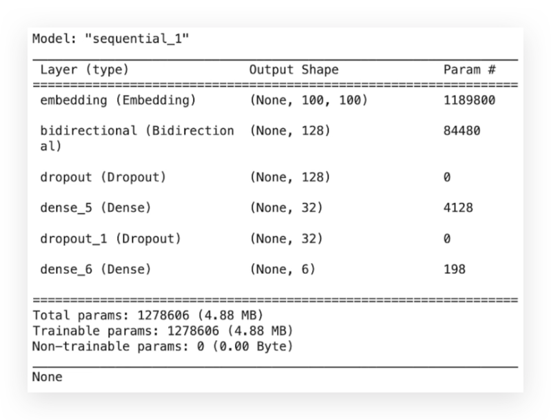
Here you can verify the layers. In version 1, we had only a dense layer. Now, we have embedding, bidirectional, dropout, and a dense layer.
Essentially, this is what you’ll observe across Deep Learning architectures. You keep adding different layers to modify the learning strategy and aim for the best possible model.
The Transformer architecture works the same way.
It introduces the attention layer, which is another component added to this stack of Deep Learning layers.
Next, we’ll convert the input data into an array format:
# 78. Define Input Data as Array
input_data = np.array(train_sequences_padded)
To ensure the data is in the proper structure, I do the same for the output data:
# 79. Define Output Data as Array
output_data = np.array(y_train_encoded)
I then prepare the hyperparameters, including the number of epochs, the train-validation split, and a patience value of 5 for early stopping:
# 80. Define Hyperparameters
num_epochs = 35  # Number of epochs
validation_split_value = 0.2  # Validation split percentage
patience = 5  # Early stopping patience
In other words, TensorFlow will wait for 5 epochs.
If the model’s performance doesn’t improve after 5 epochs, it will stop training thanks to Early Stopping:
# 81. Configure Early Stopping
early_stopping = tf.keras.callbacks.EarlyStopping(patience=patience)
I’m using a patience value of exactly 5. I can already anticipate that we’ll now see Early Stopping in action.
In other words, we won’t train for the full 35 epochs. The model will stop training earlier.
And then, we’ll have a trained model, which we’ll examine shortly.
10. Model V2 — Training and Evaluation
We set 35 epochs in command #80, correct?
And we configured early_stopping with a patience of 5.
This means that if the performance doesn’t improve for 5 consecutive passes—5 epochs—it will stop the training.
But look what happened:
# 82. Train the Model
%%time
history = model_v2.fit(
    input_data,  # Training input data
    output_data,  # Training output data
    epochs=num_epochs,  # Number of epochs
    verbose=1,  # Verbosity level
    validation_split=validation_split_value,  # Validation split ratio
    callbacks=[early_stopping]  # Callback for early stopping
)
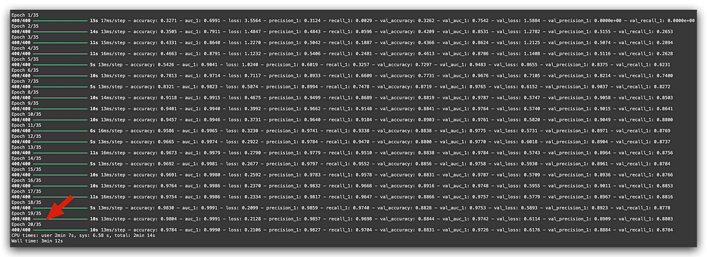
At epoch 20, the training stopped.
This is Early Stopping, a callback that’s incredibly useful for avoiding overfitting and preventing computational resource wastage.
If the model is no longer learning, why continue training? It would waste computational power and also increase the risk of overfitting.
Regarding the metrics, observe the results here:

This is the training accuracy during the first epoch: 0.32.
However, you aim for the highest possible accuracy. Look at what happens toward the very end:

0.97. The model learned! Isn’t that magnificent?
To check the other metrics, you can simply look at the notebook — they’re easier to analyze there due to the size of the visualizations. However, I can tell you this:
- The validation accuracy started at 0.32 and ended at 0.88.
- The AUC (Area Under the Curve) started at 0.75 and improved to 0.97 by the end.
The AUC ranges from 0 to 1, where higher is better. It’s generally an excellent metric for comparing models.
Now, let’s evaluate the model:
# 83. Plot Error Curves
loss, val_loss = history.history['loss'], history.history['val_loss']  # Extract training and validation loss

plt.plot(loss, label='Training Error')  # Plot training error
plt.plot(val_loss, label='Validation Error')  # Plot validation error

plt.legend()  # Add a legend
plt.show()  # Display the plot
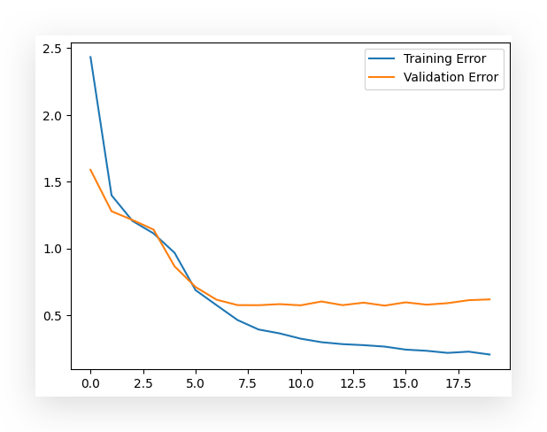
Here, I have the training and validation error curves. You can see that the validation error hasn’t dropped as much, which suggests that some adjustments could be made to further improve validation performance.
However, we still achieved excellent performance by the end.
Now, I’ll make predictions using the test data, keeping in mind that the test data must include padding:
# 84. Predictions on Test Data
predictions = model_v2.predict(test_sequences_padded)
We’ve already applied padding to the training and test data.
Now, we must use the test data (with padding) to make predictions. Next, I’ll determine the predicted labels:
# 85. Determine Predicted Labels
predicted_labels = predictions.argmax(axis=1)
Next, I’ll generate a classification report, where we expect the Precision and Recall values to be somewhat similar.
They don’t have to be identical, but if they’re close, it indicates that the model is well-balanced:
# 86. Display Classification Report
print(classification_report(y_test_le, predicted_labels))
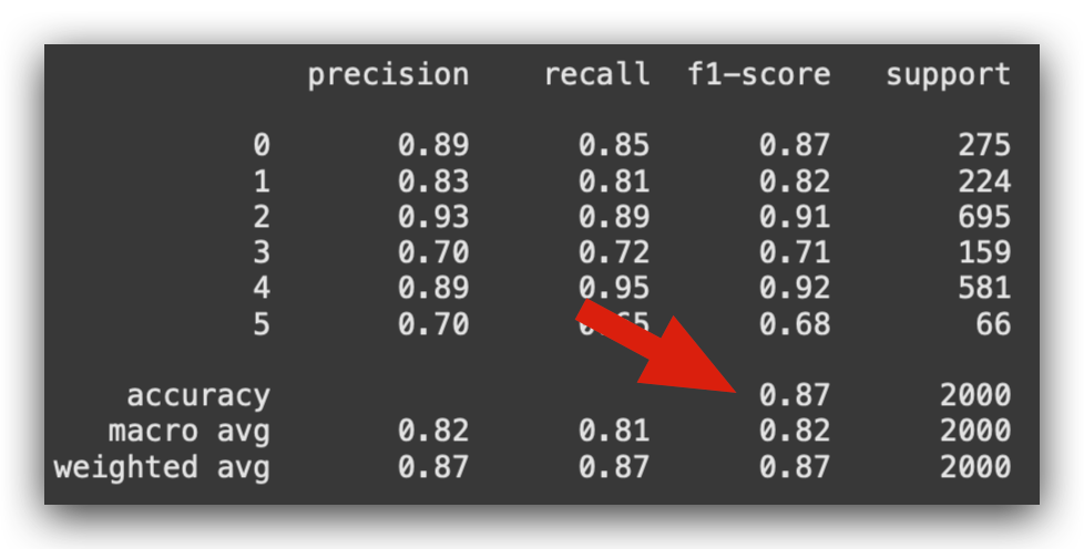
The overall performance of the model is 0.87, which is excellent.
Now, let’s display the confusion matrix, which shows the model’s errors and correct predictions:
# 87. Display Confusion Matrix
print(confusion_matrix(y_test_le, predicted_labels))
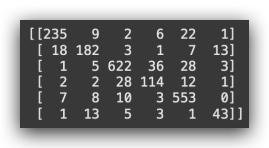
And finally, the validation accuracy is 0.88 (rounded).
# 88. Display Model Accuracy
print(accuracy_score(y_test_le, predicted_labels))

# ------> 0.8745
Then, I saved the model to disk:
# 89. Save the Model
model_v2.save('model_v2.keras')
Let’s check version 1, keeping in mind that the results may vary slightly with each execution.
Why? Because part of the process involves randomness, especially during data splitting. This is why there’s a small variation in the results every time you run the model — sometimes slightly better, sometimes slightly worse.
Now, let’s evaluate the performance of version 1:
# 42. Print Accuracy Score
print(accuracy_score(y_test_le, predictions_v1_labels))

# -----> 0.8445
0.84. Multiplying this by 100% gives 84% accuracy for version 1 of the model, which is the simplest possible architecture given the dataset and Deep Learning context.
Then, we modified the architecture and slightly adjusted the data preparation for version 2 of the model. This improved the performance on the test data to 0.87 (87%).
Key Insights:
- Increasing the model’s complexity, in this case, had a direct positive effect on performance — the model improved slightly.
- However, depending on the objective, version 1 might still be a viable option.
Why?
- Version 1 trains much faster, is simpler, easier to interpret, and only slightly less accurate.
- If your use case prioritizes maximum performance, then an LSTM (version 2) would be the obvious choice.
- On the other hand, if you value interpretability, training time, and ease of periodic retraining and saving, version 1 might be worth considering.
This is a trade-off you need to evaluate carefully based on your specific requirements.
11. Model V2 — Model Deployment
Let’s conclude version 2 of the model with a deployment procedure, so you can see how it’s done.
The process is very similar to what we did with version 1.
Since I already saved the model to disk, we can proceed as follows:
# 89. Save the Model
model_v2.save('model_v2.keras')
And now I’ll load it:
# 90. Load the Saved Model
loaded_model = load_model('model_v2.keras')
Next, I’ll use the same sentence I used in version 1.
So, let’s load the sentence:
# 91. New Sentence (Sentiment = Fear)
sentence = "i even feel a little shaky"
Convert it into a DataFrame:
# 92. Create a DataFrame with the Sentence
df_new = pd.DataFrame({'Sentence': [sentence]})
After that, apply the processing function, just as we did in version 1 of the previous tutorial:
# 93. Apply the Preprocessing Function
df_new['Processed_Sentence'] = df_new['Sentence'].apply(preprocess_text)
Next, I need to apply the same processing I used for the LSTM model. It’s the same as what I did in version 1, remember?
In version 1, I applied TF-IDF, preprocessed the data, and trained the model. Now, in version 2, we applied tokenization. So, the same must be done with the new data.
Recognizing the Pattern:
When you spot a pattern, there’s a learning opportunity. This is the pattern:
- Take your data.
- Apply the same preprocessing.
- Continue processing until it’s complete.
The processing you applied to train the model must also be applied to the new data and the test data.
Now, I’ll take the tokenizer and apply texts_to_sequences to convert the input text into its numeric representation:
# 94. Process New Data
new_sequences = tokenizer.texts_to_sequences(df_new['Processed_Sentence'])
new_sequences_padded = pad_sequences(new_sequences, maxlen=max_length)
But the model didn’t just learn from the numeric representation — it learned with padding! In fact, the model received a matrix where each row has a maximum length of 100. Each row in the matrix is padded to this length.
That’s how the model was trained, and that’s how it expects the new data, right?
So, after converting Processed_Sentence into its numeric representation, I prepared the matrix using padding, just as I did with the training data. It’s straightforward: everything you did with the training data must also be applied to the test data and new data. Same process.
- Tokenization? Done.
- Padding? Done.
Now, I’ll use the loaded model to make predictions:
# 95. Make Predictions with the Loaded Model
predictions = loaded_model.predict(new_sequences_padded)
Just make predictions using the padded data — don’t forget. Now, I’ll extract the class with the highest probability and print it for you:
# 96. Select the Class with the Highest Probability
highest_prob_class = np.argmax(predictions, axis=1)

# 97. Display the Class with the Highest Probability
highest_prob_class

# -----> array([1])
It’s class 1.
But you don’t want the number 1, you want the name of the class. So, let’s use the inverse_transformmethod of our encoder to get the class name:
# 98. Get the Class Name
class_name = label_encoder_v2.inverse_transform(highest_prob_class)
And now, the class name:
# 99. Predicted Class
class_name

Here it is. The model did a good job, achieving accurate predictions with solid performance. However, it’s a bit more complex than the first version.
It’s important to note that the data we’re working with is relatively simple. When dealing with less complex datasets, a simpler model might perform better.
Key Insight:
This highlights another pattern to keep in mind:
- Simpler data might benefit from simpler models.
- For more complex data, a simple model (like version 1) might not perform as well.
But there’s no way to know this immediately — you can’t predict it in advance. The only way to determine whether a model works is to experiment.
We’ve now experimented with two architectures. To reach the climax, the pinnacle of this journey, we’ll train a Transformer architecture.
I’ll use an LLM (Large Language Model) — specifically, one of the best in the market today: BERT, which is also multilingual.
Next Steps:
We’ll repeat this entire process but tailored to the third version of the model, which is the Transformer model.
- We’ll work with a pre-trained model.
- Then, we’ll fine-tune it using our dataset.
- Finally, we’ll evaluate whether we can achieve even better performance.
12. Model V3 Overview— Fine-Tuning
Let’s build the third and final version of the model for this project. The ultimate goal of this project is to reach version 3.
However, we introduced versions 1 and 2 to provide a basis for comparison:
- To help you understand the complexity of version 3 compared to the previous versions.
- To establish a clear understanding of how to apply a pre-trained model from the Hugging Face platform and construct a Transformer model.
In addition, we’ll fine-tune a pre-trained model using the concept of transfer learning.
First, let me provide an overview. I’ll use the data processed with Spacy:
# 100. Display Data Processed with SpaCy
training_data.head()

The input data for version 3 will be the same as those used for versions 1 and 2.
Next, we’ll create a function for encoding, which is essentially the tokenization process. However, this time it will be customized to match the characteristics of the pre-trained model we’ll use:
# 101. Function to Encode Text into Integer Sequences for BERT Input
def encode_texts(texts, tokenizer, chunk_size=256, maxlen=512):

    # 101.a Configure the tokenizer to truncate texts to the specified maximum length
    tokenizer.enable_truncation(max_length=maxlen)

    # 101.b Configure the tokenizer to apply padding up to the specified maximum length
    tokenizer.enable_padding(length=maxlen)

    # 101.c List to store input IDs generated by the tokenizer
    input_ids = []

    # 101.d List to store attention masks generated by the tokenizer
    attention_masks = []

    # 101.e Iterate over the texts in chunks of the specified chunk_size
    for i in tqdm(range(0, len(texts), chunk_size)):

        # 101.f Select a chunk of texts to process
        text_chunk = texts[i:i+chunk_size].tolist()

        # 101.g Encode the text chunk in batches using the tokenizer
        encs = tokenizer.encode_batch(text_chunk)

        # 101.h Add the encoded input IDs to the input_ids list
        input_ids.extend([enc.ids for enc in encs])

        # 101.i Add the generated attention masks to the attention_masks list
        attention_masks.extend([enc.attention_mask for enc in encs])

    # 101.j Return the input IDs and attention masks as numpy arrays
    return np.array(input_ids), np.array(attention_masks)
See, I’m introducing the third data processing strategy:
- I used TF-IDF in version 1,
- The standard Keras tokenizer in version 2,
- And now, I’ll create a custom tokenizer with you.
Next, I’ll load the pre-trained model, starting with the tokenizer:
# 102. Load the Pre-Trained Model's Tokenizer
bert_tokenizer = transformers.DistilBertTokenizer.from_pretrained(
'distilbert-base-multilingual-cased')

Every pre-trained model comes with its own tokenizer. For each version I created, I prepared the data differently, right?
When deploying the model, you must apply the same strategy to new data. Isn’t this what I already demonstrated in versions 1 and 2?
It’s the same principle here. Now, I’m using a model that someone else created — the pre-trained model. For them to create this model, they applied tokenization, and they provide the tokenizer for you.
When you access the Hugging Face platform — which I’ll show you shortly — you’ll notice that the pre-trained model is typically accompanied by its tokenizer. Why? Because that’s how the model was trained.
This proves the point I’ve been emphasizing throughout this tutorial.
Next, I’ll save the model and its vocabulary to disk:
# 103. Save the Tokenizer and Vocabulary Locally
bert_tokenizer.save_pretrained('.')
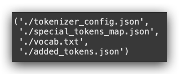
The vocabulary of this pre-trained BERT model is quite heavy. So, what will I do? I’ll use a lighter tokenizer, which is also provided by Keras:
# 104. Load a Faster Tokenizer Using the Main Tokenizer's Vocabulary
# from tokenizers import BertWordPieceTokenizer
fast_tokenizer = BertWordPieceTokenizer('vocab.txt', lowercase=False)
This tokenizer will read the vocabulary but will be slightly faster, speeding up the training process.
This is where the expertise of an AI engineer comes in — knowing how to optimize the process to train the model in the shortest time possible.
Next, I’ll split the training data into training and validation sets:
# 106. Split Data into Training and Validation Sets with Stratified Sampling

# Processed text for training
X_train, X_valid, Y_train, Y_valid = train_test_split(
    training_data['processed_text'].values,

    # Sentiment labels for training
    training_data['sentiment'].values,

    # Validation split ratio
    test_size=0.2,

    # Random state for reproducibility
    random_state=42,

    # Stratified sampling by sentiment labels
    stratify=training_data['sentiment']
)
This is more important than ever when training a large language model, as is the case here.
I’ll limit the model to a maximum sequence length of 100:
# 107. Define Maximum Length for Texts
max_length = 100
For example, as I did with LSTM.
Although the BERT model can handle longer sequences, I’ll keep the sequence length similar to version 2. This allows us to see if the model can deliver better performance under the same conditions.
Now, I’ll encode the data:
# 108. Apply Encoding (Tokenization) to the Data
X_train_final, train_mask = encode_texts(X_train, fast_tokenizer, maxlen=max_length)
X_valid_final, valid_mask = encode_texts(X_valid, fast_tokenizer, maxlen=max_length)
X_test_final, test_mask = encode_texts(test_data['processed_text'].to_numpy(), fast_tokenizer, maxlen=max_length)

This is the tokenization. Next, we need to encode the target variable:
# 110. Define the Encoder for Output Data
label_encoder_v3 = LabelEncoder()
I’ll now define the batch size:
# 113. Define Batch Size
BATCH_SIZE = 16
And here’s a specific characteristic: for this pre-trained model, I need to prepare the data in TensorFlow’s dataset format.
Here’s how to do it:
# 114. Prepare the Training Dataset in the Format Expected by TensorFlow

# Combine inputs and labels
train_dataset = (
    tf.data.Dataset
    .from_tensor_slices(((X_train_final, train_mask), y_train_encoded))

    # Repeat the dataset for multiple epochs
    .repeat()

    # Shuffle the data with a buffer size of 2048
    .shuffle(2048)

    # Group data into batches of the specified size
    .batch(BATCH_SIZE)
)
These are the complications humans like to create! So, I’ll prepare the specific format. After that, I’ll define a function to create the model:
# 117. Function to Create the Model
def create_model(transformer, max_len=512):

    # 117.a Input layer for word IDs
    input_word_ids = tf.keras.layers.Input(
        shape=(max_len,), dtype=tf.int32, name="input_word_ids"
    )

    # 117.b Input layer for attention masks
    attention_mask = tf.keras.layers.Input(
        shape=(max_len,), dtype=tf.int32, name="attention_mask"
    )

    # 117.c Custom layer for the Transformer
    sequence_output = TransformerLayer(transformer)(
        [input_word_ids, attention_mask]
    )

    # 117.d Select the CLS token (first token)
    cls_token = sequence_output[:, 0, :]

    # 117.e Dense layer with softmax activation for classification
    out = Dense(6, activation="softmax")(cls_token)

    # 117.f Keras model definition
    model = tf.keras.Model(
        inputs=[input_word_ids, attention_mask], outputs=out
    )

    # 117.g Compile the model
    model.compile(
        optimizer=Adam(learning_rate=1e-5),
        loss="categorical_crossentropy",
        metrics=["accuracy", Precision(), Recall(), AUC()],
    )

    return model
This function will take the pre-trained model, remove its head, and add our custom head. Why? So it can learn from our data and patterns for the sentiment analysis we’re conducting.
Now, I’ll import the layers from the pre-trained Transformer model:
# 119. Load the Pre-Trained Model
transformer_layer = TFDistilBertModel.from_pretrained(
    "distilbert-base-multilingual-cased"
)
Next, I’ll create the model:
# 120. Create the Model with the Pre-Trained Transformer Layers and Custom Layers for Fine-Tuning
model_v3 = create_model(transformer_layer, max_len=max_length)
I’ll generate the summary and freeze some layers of the model:
# 121. Display Model Summary
model_v3.summary()

# 122. Set the First Three Layers of the Model as Non-Trainable
model_v3.layers[0].trainable = False
model_v3.layers[1].trainable = False
model_v3.layers[2].trainable = False
Why? Because I don’t want to train the entire model. I only want to train the head, the final part. So, I’ll freeze some layers.
After that, I’ll generate another summary:
# 123. Display Updated Model Summary
model_v3.summary()
Let’s prepare the hyperparameters and train the model:
# 124. Define Hyperparameters
n_steps = X_train_final.shape[0] // BATCH_SIZE  # Number of steps per epoch
num_epochs = 3  # Number of epochs

# 125. Train the Model
%%time
history = model_v3.fit(
    train_dataset,  # Training dataset
    steps_per_epoch=n_steps,  # Number of steps per epoch
    validation_data=valid_dataset,  # Validation dataset
    epochs=num_epochs  # Number of epochs
)
After training the model, the remaining steps are essentially the same as in the previous versions.
I’ll evaluate the model and deploy it at the end, following the same pattern.
With that, we’ll have the entire project completed.
13. Model V3 — Custom Tokenization Function
For version 3 of the model, I’ll use the same input data as in versions 1 and 2 — data that has already undergone some preprocessing with Spacy.
What’s the purpose of Spacy?
Spacy is used to clean the data and apply initial preprocessing to text data, such as:
- Removing unnecessary elements.
- Applying lemmatization or stemming to reduce words to their root forms.
This preprocessing serves as the starting point. Afterward, further processing depends on the architecture of the model.
Spacy’s preprocessing — such as cleaning and lemmatizing — is sufficient because the models are already showing good performance. While additional preprocessing with Spacy could be done, it’s not strictly necessary here.
Next Step: Tokenization
From this point, I’ll create a custom function for tokenization, referred to as encoding:
# 101. Function to Encode Text into Integer Sequences for BERT Input
def encode_texts(texts, tokenizer, chunk_size=256, maxlen=512):

    # 101.a Configure the tokenizer to truncate texts to the specified maximum length
    tokenizer.enable_truncation(max_length=maxlen)

    # 101.b Configure the tokenizer to apply padding up to the specified maximum length
    tokenizer.enable_padding(length=maxlen)

    # 101.c List to store input IDs generated by the tokenizer
    input_ids = []

    # 101.d List to store attention masks generated by the tokenizer
    attention_masks = []

    # 101.e Iterate over the texts in chunks of the specified chunk_size
    for i in tqdm(range(0, len(texts), chunk_size)):

        # 101.f Select a chunk of texts to process
        text_chunk = texts[i:i+chunk_size].tolist()

        # 101.g Encode the text chunk in batches using the tokenizer
        encs = tokenizer.encode_batch(text_chunk)

        # 101.h Add the encoded input IDs to the input_ids list
        input_ids.extend([enc.ids for enc in encs])

        # 101.i Add the generated attention masks to the attention_masks list
        attention_masks.extend([enc.attention_mask for enc in encs])

    # 101.j Return the input IDs and attention masks as numpy arrays
    return np.array(input_ids), np.array(attention_masks)
Unfortunately, there’s no standard naming convention in AI or Data Science. Everyone uses their own terminology.
Over time, you realize it doesn’t matter much. If you understand the concept, the naming isn’t a big deal.
What is Tokenization?
Tokenization is converting words into numbers. This is the concept of encoding.
- I’m performing tokenization for the input data.
- For the output data, I’m doing encoding.
Custom Tokenization Function
We’re preparing a custom function for this. The function will:
- Accept text data, the tokenizer, a chunk size (default: 256), and a maximum length (default: 512, which is the maximum BERT can process).
- Activate truncation for the specified max_length.
What is Truncation?
It limits sequences to a specific maximum length. In our case, the maximum will be 100, the same size used in version 2.
Here’s the implementation:
# 101.a Configure the tokenizer to truncate texts to the specified maximum length
    tokenizer.enable_truncation(max_length=maxlen)
After that, padding will be enabled. This is the same concept as in V2.
Were all sentences the same length? No. But the matrix must have uniform dimensions. So, padding will fill the empty spots with a character, usually the value 0:
# 101.b Configure the tokenizer to apply padding up to the specified maximum length
 tokenizer.enable_padding(length=maxlen)
After that, initialize a list to store the encoded IDs, which involves converting the text into numeric values:
# 101.c List to store input IDs generated by the tokenizer
 input_ids = []
I’ll then create a loop using TQDM to show a progress bar, making it visually appealing and allowing you to see the process in action:
# 101.e Iterate over the texts in chunks of the specified chunk_size
 for i in tqdm(range(0, len(texts), chunk_size)):
I create a chunk of the text:
# 101.f Select a chunk of texts to process
 text_chunk = texts[i:i+chunk_size].tolist()
So, I take my text dataset, which was received as input, extract a chunk, and then apply the tokenizer:
# 101.g Encode the text chunk in batches using the tokenizer
 encs = tokenizer.encode_batch(text_chunk)
This tokenizer, which will be passed as a parameter, will be the pre-trained BERT tokenizer that I’ll extract from Hugging Face.
After that, I’ll extend the list with the encoded IDs:
# 101.h Add the encoded input IDs to the input_ids list
        input_ids.extend([enc.ids for enc in encs])

        # 101.i Add the generated attention masks to the attention_masks list
        attention_masks.extend([enc.attention_mask for enc in encs])

# 101.j Return the input IDs and attention masks as numpy arrays
return np.array(input_ids), np.array(attention_masks)
This is essentially about expanding the dimensions. And that’s it — by the end, we’ll have the tokenized text.
It’s a way to parametrize the process.
- In version 1, I used TF-IDF.
- In version 2, I introduced the standard Keras tokenizer, useful for LSTM.
- And now, in version 3, I’m introducing a customized process.
14. Model V3 — Loading the Tokenizer from Hugging Face
We’ve already built our customized function.
Next, we’ll download the tokenizer. I’ll head over to Hugging Face and download the tokenizer for this model:

Why This Model?
This is a BERT model, pre-trained, but it’s also multilingual. This means you can easily adapt this project to your own data in up to 104 different languages, as this model supports multiple languages.
When using a pre-trained model, your job is to visit Hugging Face and select one of the many options it offers. In fact, new pre-trained models are added almost daily — actually, every day!
Here’s the process:
- Search: Go to Hugging Face and browse for a suitable pre-trained model for your task.
- Select: Choose a model that fits your needs.
- Download: Expect the model to come with a tokenizer (most do).
- Prepare Data: Use the tokenizer to preprocess your data and prepare it for training.
- Fine-Tuning (Optional): Decide if you need to fine-tune the model for your specific dataset.
By following these steps, you can quickly leverage powerful pre-trained models like BERT for various tasks, including sentiment analysis, across multiple languages.
distilbert/distilbert-base-multilingual-cased · Hugging Face
Let’s visit the Hugging Face page for this model.
Last month alone, this model had over 300,000 downloads:
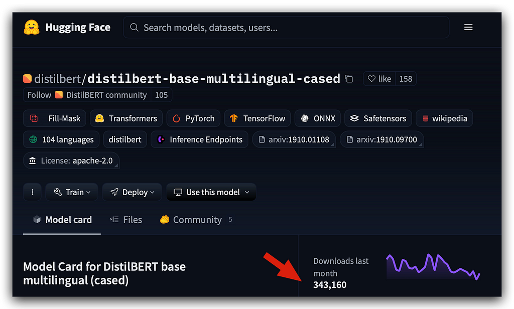
BERT is an LLM (Large Language Model). It is smaller than other LLMs but highly efficient and extremely useful for NLP tasks (Natural Language Processing).
The version I’m using is DistilBERT, a lighter variant that has been customized to work with TensorFlow.
Many language models were originally trained with PyTorch, but efforts are being made to prepare these models for TensorFlow as well. This model is one of those adaptations, and it is also multilingual.

In other words, you can adapt this project to up to 104 languages, and BERT can be used effortlessly.
Here, you’ll find details about the authors and the research paper. There is a wealth of material available on Hugging Face.
What I want to point out is located in the Files and Versions section:
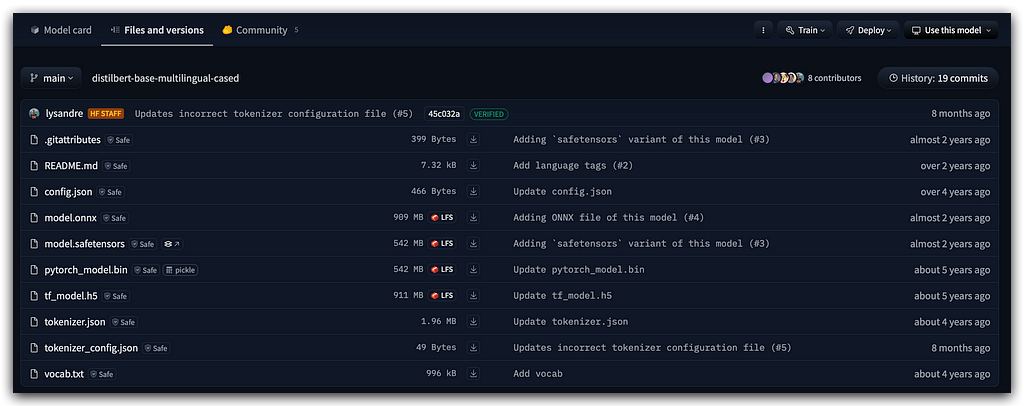
This is the model and tokenizer. Where’s the model? It’s the tf_model.h5 file for TensorFlow.
You also have the model for PyTorch, along with the vocab.txt file and tokenizer.json, which store the vocabulary and tokenizer configuration. Everything is ready to go.
Key Point:
You can only use this model if you apply the same tokenizer. Why? Because this tokenizer was used to train the model.
If you’re going to use the model, you must use the same tokenizer.
Saving Your Tokenizer:
Does that mean that when you create your own model, you’ll need to save your tokenizer?
Yes, of course! That’s exactly how it works.
Next Step:
The next step is to use the Transformers package, which connects to Hugging Face to load the model and tokenizer.
# 102. Load the Pre-Trained Model's Tokenizer
bert_tokenizer = transformers.DistilBertTokenizer.from_pretrained(
    'distilbert-base-multilingual-cased')
Let’s fetch the distilbert-base-multilingual-cased model. From this pre-trained model, we’ll also load the tokenizer.
The progress bar will indicate the download process:

And then, I’ll save all of this to disk. Why? Because I’ll need to use the vocabulary later.
Here’s how to save both the model and tokenizer locally:.
# 103. Save the Tokenizer and Vocabulary Locally
bert_tokenizer.save_pretrained('.')
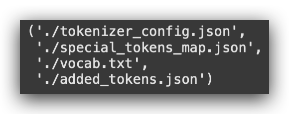
Notice that now I have the tokenizer, which is a JSON file. I also have a special mapping file, the vocabulary, and another file.
Go to the side panel, refresh Google Colab, and check the left sidebar to see that everything has already been downloaded.
15. Model 3 — Improving Tokenizer Performance
Let’s use a faster tokenizer. This will speed up the training process while still achieving good performance in the end:
# 104. Load a Faster Tokenizer Using the Main Tokenizer's Vocabulary
# from tokenizers import BertWordPieceTokenizer
fast_tokenizer = BertWordPieceTokenizer('vocab.txt', lowercase=False)
I’ve located the package where this function comes from. It’s already imported at the top of the notebook.
I’ve included it here as a reference, so you don’t have to scroll all the way back up, especially since we’re now working with over 100 cells.
I’m importing the function and instructing it to create a faster tokenizer based on the vocab.txt file.
Key Point:
You cannot create your own vocabulary. It must be the same vocabulary used to train the pre-trained BERT model.
Researchers created and trained the model using this vocabulary, so you must use the same one for your tokenizer.
Now, let’s execute the fast_tokenizer:
# 105. Visualize the Tokenizer
fast_tokenizer

Notice that I now have the vocabulary size, the model, the start token, and the separator token — all of this comes from BERT’s vocabulary.
In other words, these were used during the data preparation process to train the model.
Now, I have the fast_tokenizer, which will significantly speed up the process.
I’ll use this fast_tokenizer shortly when applying it to the training, validation, and test data.
16. Model V3 — Data Preparation
Let’s complete the data preparation, followed by fine-tuning and then training the model.
In all three versions, I’ve consistently used validation data. Did you notice?
- In version 1 and version 2, we split the training data into training and validation sets.
- Why? Because in Deep Learning, this is crucial.
Since these models are typically deeper and heavier, it’s beneficial to evaluate them during training using validation data.
This approach also allows you to use callbacks, such as early stopping, to halt training when improvements plateau.
For version 3, I’m applying the same strategy: splitting data into training and validation sets.
- In version 1, I split the data one way.
- In version 2, I used a slightly different method.
- Now, I’m presenting yet another way:
# 106. Split Data into Training and Validation Sets with Stratified Sampling

# Processed text for training
X_train, X_valid, Y_train, Y_valid = train_test_split(
    training_data['processed_text'].values,

    # Sentiment labels for training
    training_data['sentiment'].values,

    # Validation split ratio
    test_size=0.2,

    # Random state for reproducibility
    random_state=42,

    # Stratified sampling by sentiment labels
    stratify=training_data['sentiment']
I’m using stratified sampling, which I also used in version 1, by the way. The notebook includes an explanation of exactly what this strategy entails.
Here’s the maximum length I’ll be using:
# 107. Define Maximum Length for Texts
max_length = 100
his was my choice. If you want to change the length, no problem — BERT supports longer sequences.
But be careful!
Typically, to define the maximum length, you check the longest sentence in your dataset. For example:
- If the longest sentence is 100, you set the max length to 100.
- You won’t have anything longer than 100, but you’ll have many shorter sentences.
- These shorter ones will be padded, as we’ve seen before.
However, it’s not always feasible to use the longest sentence. Sometimes, the longest sentence is too large, which results in a huge input matrix.
In such cases, it’s better to apply truncation, as I showed you with the parameter in version 2.
Here, I’ll work with a length of 100 and proceed to apply encoding or tokenization:
# 108. Apply Encoding (Tokenization) to the Data
X_train_final, train_mask = encode_texts(X_train, fast_tokenizer, maxlen=max_length)
X_valid_final, valid_mask = encode_texts(X_valid, fast_tokenizer, maxlen=max_length)
X_test_final, test_mask = encode_texts(test_data['processed_text'].to_numpy(), fast_tokenizer, maxlen=max_length)

Once you understand the concept, it becomes much easier to work with any nomenclature. That’s what I’m aiming to do here with you.
In this case, I’ll apply the encode_texts, which is our custom function, and use the fast_tokenizer for tokenization.
Notice that I’m applying this to the training, validation, and test data, all using the maximum length we just defined.
Let’s take a look at the shape of the input data for training:
# 109. Check Shape of Final Training Data
X_train_final.shape

# -----> (12800, 100)
And there it is: 12,800 x 100, which is the maximum size. This means there won’t be any sequences larger than this.
Next, I’ll apply the encoder, which is the encoding of the target variable:
# 110. Define the Encoder for Output Data
label_encoder_v3 = LabelEncoder()
Just like we did in versions 1 and 2, we create the encoder, apply it, and remember to use fit_transform for the training set and transform for validation and test sets:
# 111. Apply the Encoder (fit_transform only on Training Data)
y_train_le = label_encoder_v3.fit_transform(Y_train)
y_valid_le = label_encoder_v3.transform(Y_valid)
y_test_le = label_encoder_v3.transform(test_data['sentiment'])
After that, convert the target variable into a categorical variable:
# 112. Convert Output Variable to Categorical
y_train_encoded = to_categorical(y_train_le)
y_valid_encoded = to_categorical(y_valid_le)
y_test_encoded = to_categorical(y_test_le)
I’ll use a batch size of 16:
# 113. Define Batch Size
BATCH_SIZE = 16
Why 16? You can’t load all the data into memory at once. Instead, you process it in batches, piece by piece, batch by batch.
I’m using 16 because it provides good performance. Feel free to experiment with other values later.
When working with TensorFlow and the function I’ll use with BERT, the data needs to be in the tf.data.Datasetformat:
# 114. Prepare the Training Dataset in the Format Expected by TensorFlow

# Combine inputs and labels
train_dataset = (
    tf.data.Dataset
    .from_tensor_slices(((X_train_final, train_mask), y_train_encoded))

    # Repeat the dataset for multiple epochs
    .repeat()

    # Shuffle the data with a buffer size of 2048
    .shuffle(2048)

    # Group data into batches of the specified size
    .batch(BATCH_SIZE)
)
I’ll prepare the data by slicing tensors.
Essentially, this modifies the dimensions of the tensors (which are matrices), performs shuffling, and applies the batch size. This will prepare the training dataset, validation dataset, and test dataset.
At this point, the data is ready for the pre-trained model we’re working with in version 3.
Can We Use the Pre-Trained Model Directly?
Yes, we could. You’re not required to train or fine-tune a pre-trained model. Is that clear?
The pre-trained model is ready to use as it is. The question, however, is whether the pre-trained model is suitable for your specific use case.
Use Case in Our Example:
Our goal is sentiment classification on text.
- BERT wasn’t specifically trained for this task.
- So, we need to adapt it to this use case.
Next Steps:
- I’ll leverage the pre-trained model, but I’ll cut off the head and add a new head tailored to sentiment classification.
- The model will then be fine-tuned using our data.
- I’ll train only the final part (the new head), which will make the training process much faster.
By doing this, we expect to achieve a model with good performance for our specific use case.
17. Model V3 — Custom Function for Fine-Tuning
Let’s move on to the fine-tuning of our model, the highlight of this project.
Here’s the function:
# 117. Function to Create the Model
def create_model(transformer, max_len=512):

    # 117.a Input layer for word IDs
    input_word_ids = tf.keras.layers.Input(
        shape=(max_len,), dtype=tf.int32, name="input_word_ids"
    )

    # 117.b Input layer for attention masks
    attention_mask = tf.keras.layers.Input(
        shape=(max_len,), dtype=tf.int32, name="attention_mask"
    )

    # 117.c Custom layer for the Transformer
    sequence_output = TransformerLayer(transformer)(
        [input_word_ids, attention_mask]
    )

    # 117.d Select the CLS token (first token)
    cls_token = sequence_output[:, 0, :]

    # 117.e Dense layer with softmax activation for classification
    out = Dense(6, activation="softmax")(cls_token)

    # 117.f Keras model definition
    model = tf.keras.Model(
        inputs=[input_word_ids, attention_mask], outputs=out
    )

    # 117.g Compile the model
    model.compile(
        optimizer=Adam(learning_rate=1e-5),
        loss="categorical_crossentropy",
        metrics=["accuracy", Precision(), Recall(), AUC()],
    )

    return model
Now, fine-tuning will seem so simple that you might say, “Is that all?” Why? Because we’ve been building this knowledge step by step, from the very beginning of this project.
Let’s take a look at what we’re doing in fine-tuning.
We’ll create a function that takes the Transformer (pre-trained model) as input.
- What is the Transformer? It’s the pre-trained model.
- The model will be passed as an argument to this function.
If I don’t change the sequence length, it will default to 512, which is the standard for BERT.
Next, I’ll define the input layer with the maximum sequence length:
# 117.a Input layer for word IDs
    input_word_ids = tf.keras.layers.Input(
        shape=(max_len,), dtype=tf.int32, name="input_word_ids"
    )
I’m using the Input layer from Keras to define the input. The shape is set to (max_len,), which corresponds to the maximum sequence length.
The data type is defined as int32, as the input will consist of integer token IDs.
Finally, I name the input layer input_word_ids for clarity and organization in the model architecture.
# 117.c Custom layer for the Transformer
    sequence_output = TransformerLayer(transformer)(
        [input_word_ids, attention_mask]
    )
I will then obtain the sequence output from the Transformer.
The Transformer is a pre-trained model, and I’ll use its output along with my input_word_ids. This forms the sequence output.
Right after that, I’ll extract the CLS token, which represents the classification token:
 # 117.d Select the CLS token (first token)
    cls_token = sequence_output[:, 0, :]
The CLS token is a specific feature of BERT.
BERT was trained with text data for text classification tasks, and it includes a special token called CLS to mark the start of each sequence. This token is what I need to extract and use during training.
At this point, we’ve essentially completed the Transformer integration. This is the part of the pre-trained model that will be used in our final architecture:
# 117. Function to Create the Model
def create_model(transformer, max_len=512):

    # 117.a Input layer for word IDs
    input_word_ids = tf.keras.layers.Input(
        shape=(max_len,), dtype=tf.int32, name="input_word_ids"
    )

    # 117.b Input layer for attention masks
    attention_mask = tf.keras.layers.Input(
        shape=(max_len,), dtype=tf.int32, name="attention_mask"
    )

    # 117.c Custom layer for the Transformer
    sequence_output = TransformerLayer(transformer)(
        [input_word_ids, attention_mask]
    )

    # 117.d Select the CLS token (first token)
    cls_token = sequence_output[:, 0, :]
From here, I’ll add my head, which in this case is the final layer of the model. This will be a dense layer:
# 117.e Dense layer with softmax activation for classification
    out = Dense(6, activation="softmax")(cls_token)
Why the number 6? Because we have 6 classes in the output variable. Essentially, I’m adding a new head to the model, instructing it to deliver 6 predictions.
When I load the Transformer later, I’ll freeze the initial layers. These initial layers won’t be modified because they are already pre-trained.
The pre-trained model, which I’ll load shortly, contains the essence — the core of the model. I’ll keep these weights intact and only modify the head, which is what I’m doing here by adding a dense layer.
Notice the importance of the first version of the model. What did I do in version 1? I worked solely with a dense layer.
As I mentioned then, dense layers are used in almost every Deep Learning architecture. At some point, there will always be a dense layer.
In this case, it’s the last layer, responsible for applying the Softmax activation, which provides the probabilities for each class. Using the CLS token (BERT’s special classification token), I’ll now construct the full model.
Here’s how I’ll build it: using the inputs from the Transformer (the first layers) and the new head, named out:
# 117.f Keras model definition
    model = tf.keras.Model(
        inputs=[input_word_ids, attention_mask], outputs=out
    )
Done. What I’m essentially telling Keras is that I’ll use the body of the Transformer along with a custom head.
This custom head is now adjusted to fit my data and tailored to my use case. I’ll train this shortly, but only the new head. I’m not going to train the entire model from scratch.
Why? Because I already have a set of pre-trained layers that are ready to use.
Here’s the corresponding code:
    # 117.a Input layer for word IDs
    input_word_ids = tf.keras.layers.Input(
        shape=(max_len,), dtype=tf.int32, name="input_word_ids"
    )

    # 117.b Input layer for attention masks
    attention_mask = tf.keras.layers.Input(
        shape=(max_len,), dtype=tf.int32, name="attention_mask"
    )

    # 117.c Custom layer for the Transformer
    sequence_output = TransformerLayer(transformer)(
        [input_word_ids, attention_mask]
    )

    # 117.d Select the CLS token (first token)
    cls_token = sequence_output[:, 0, :]

    # 117.e Dense layer with softmax activation for classification
    out = Dense(6, activation="softmax")(cls_token)

    # 117.f Keras model definition
    model = tf.keras.Model(
        inputs=[input_word_ids, attention_mask], outputs=out
    )
This is fine-tuning. If I had shown you only this part of the project, it wouldn’t have been as engaging, right? Now, you understand what we’re doing.
- In version 1, I built a complete architecture.
- In version 2, I built another complete architecture and trained it from scratch.
- In both cases, I trained the model from zero.
Now, it’s different. I’m taking a pre-trained model, using its first layers, adding a new head, and training only the final part.
This is fine-tuning, where we adapt an excellent pre-trained model to our specific use case.
Could I train BERT from scratch? Yes, absolutely. But to do so, you’d need an enormous amount of data. Do you have access to such a dataset? Likely not. But do you even need it?
For this sentiment classification task, the dataset I have is sufficient. I can create a model capable of classifying this data without starting from scratch.
If your use case is covered, why train from scratch? The only reason would be if you want to customize the architecture further. However, training from scratch comes with costs. Training large models like BERT is expensive — it’s not free.
For companies, the key question becomes:
- Does it justify the cost?
- Is it worth the effort?
If yes, then fine — train from scratch. But this is becoming increasingly uncommon. Why? Because using pre-trained models is easier, faster, and cheaper. You adapt them to your use case, as I’ve demonstrated here.
Finally, we also need to compile the model:
# 117.g Compile the model
  model.compile(
    optimizer=tf.keras.optimizers.Adam(learning_rate=1e-5),  # Small learning rate for fine-tuning
    loss="categorical_crossentropy",  # Suitable for multi-class classification
    metrics=["accuracy"]  # Metric for evaluation
)

    return model
Exactly like any other model, right? I’ll use the Adam optimizer, with a learning rate, the categorical_crossentropy loss function — just like I did in the previous version — and the same metrics.
And that’s it. You create the function, and the fine-tuning function is successfully created
18. Model V3 — Loading the Pre-Trained Model from Hugging Face
The Hugging Face platform is full of pre-trained Transformer models. There are countless models available, making it a playground for anyone interested in Deep Learning.
You browse the site, find the model you need, load it, and don’t forget to also load the tokenizer. Then, you customize it to adapt it to your specific use case, just as I’m doing with you in this project.
How to Load a Pre-Trained Model:
You use the Transformers library (the Python package) to connect directly to Hugging Face:
# 119. Load the Pre-Trained Model
transformer_layer = TFDistilBertModel.from_pretrained(
    "distilbert-base-multilingual-cased")
You specify the model you want to use. In this case, I’m using TFDistilBertModel, which is the TensorFlow version. If you were using PyTorch, you would need to find the corresponding function for PyTorch.
How Do You Find the Correct Function or Attribute?
You need to visit the Transformers documentation. Search for the exact function name that corresponds to the model you want to use.
For example, if you’re working with TensorFlow, you’ll use TFDistilBertModel. If it’s PyTorch, the function would be different.
Once you’ve found the appropriate function, you simply call from_pretrained and provide the specific model address from Hugging Face:
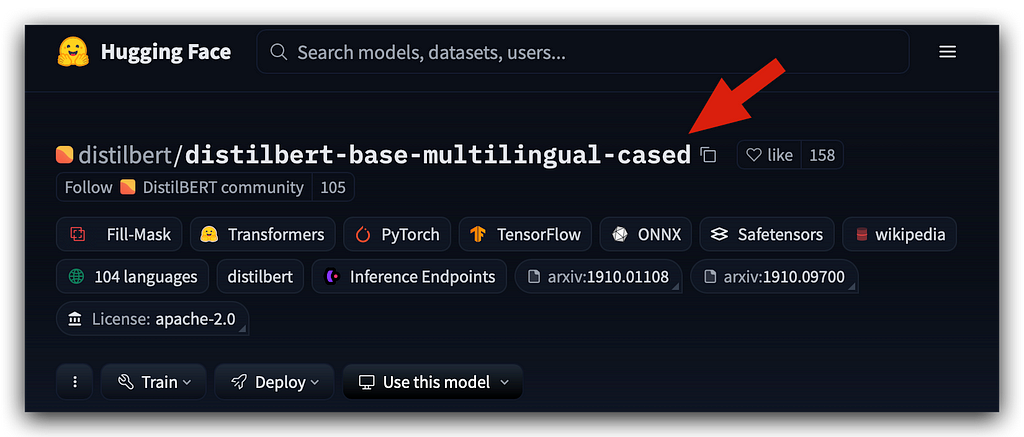
This is the name you use. There’s even an icon here for you to copy the name.
So, you’ll copy the name displayed on the Hugging Face platform.
What’s the purpose of this name? It serves as the address for the Transformers Python package to connect to the Hugging Face repository and fetch the files you need, whether it’s the tokenizer or the model.
In our case, I want the model — specifically the file designed for TensorFlow (TF).
# 119. Load the Pre-Trained Model
transformer_layer = TFDistilBertModel.from_pretrained(
    "distilbert-base-multilingual-cased")
So, in this case, I’m loading the model. The pre-trained model will be our Transformer layer.
Everything is described in the notebook for you, so make sure to read through it for further details. Now, let’s execute it.

Notice that it downloads the files. Keep in mind that when your Google Colab session expires, everything you’ve done is lost.
Your goal is to create the model, so you should save the file to disk. I’ll show you how to save the Transformer model as well.
But remember, anything done in Colab will be lost after the session expires.
By the way, a message will appear indicating that with PyTorch, the model hasn’t been initialized, etc. It’s just a warning, no issue. You can proceed.
Next, we create the model.
# 120. Create the Model with the Pre-Trained Transformer Layers and Custom Layers for Fine-Tuning
model_v3 = create_model(transformer_layer, max_len=max_length)
Notice that I will call that custom function.
I will call the transformer_layer, which is what I just imported, along with the maximum length. This will create the model architecture.
Let’s summarize:
# 121. Display Model Summary
model_v3.summary()
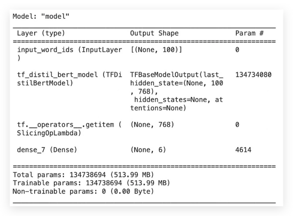
I will now freeze the inner layers because what I really want is to train the final part of the model.
This is a strategy when working with Transfer Learning.
# 122. Set the First Three Layers of the Model as Non-Trainable
model_v3.layers[0].trainable = False
model_v3.layers[1].trainable = False
model_v3.layers[2].trainable = False
If you don’t freeze the inner layers, what will happen? It will retrain from scratch.
But that’s exactly what I’m trying to avoid, okay? Because if I train from scratch, I’ll need a much larger dataset than I currently have. So it doesn’t make sense.
Therefore, I need to freeze the inner layers. And that’s what we’re doing here by setting trainable = False. There’s also a description for you in the notebook—make sure to read it later.
Now, I have the summary of the final version of our model:
# 123. Display Updated Model Summary
model_v3.summary()
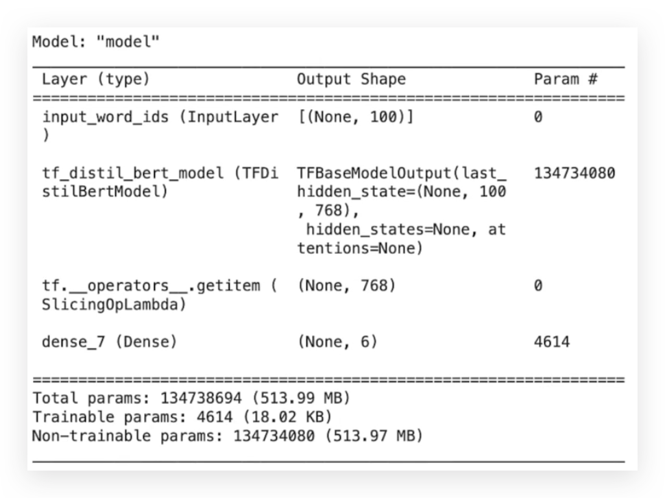
And next, we define the hyperparameters
# 124. Define Hyperparameters
n_steps = X_train_final.shape[0] // BATCH_SIZE  # Number of steps per epoch
num_epochs = 3  # Number of epochs
The number of steps and the number of epochs — only three. Yes, only three epochs are enough to prepare this model.
19. Model V3 — Training and Evaluation of the Fine-Tuned Model
Now, I have the training of the model in version 3:
# 125. Train the Model
%%time
history = model_v3.fit(
    train_dataset,  # Training dataset
    steps_per_epoch=n_steps,  # Number of steps per epoch
    validation_data=valid_dataset,  # Validation dataset
    epochs=num_epochs  # Number of epochs
)
Notice that it took 2 minutes and 18 seconds. We started with a low accuracy during training, and then it increased, indicating that the model was learning.
Look at the AUC — the same trend. It started at 97, went up to 98, and reached 99.
In a moment, I’ll do the full comparison, but clearly, this version performed better than the other two, achieving better results.
Now, let’s check the metrics:
# 126. Plot Learning Curves
loss, val_loss = history.history['loss'], history.history['val_loss']  # Extract training and validation loss

plt.plot(loss, label='Training Error')  # Plot training error
plt.plot(val_loss, label='Validation Error')  # Plot validation error

plt.legend()  # Add a legend
plt.show()  # Display the plot
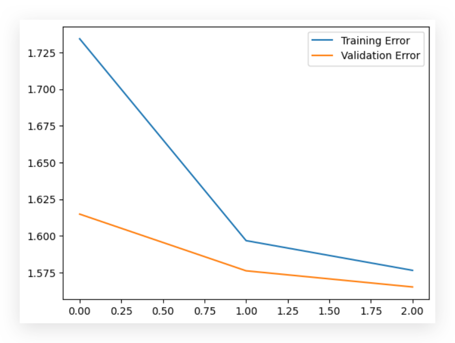
Here’s the graph showing the learning curve for training and validation.
It starts high and then drops. You can observe that in validation, it remains almost on a plateau.
In other words, with just three epochs, you can fine-tune a pre-trained model and solve your business problem, achieving a model with good predictive capability.
After that, make predictions with the test data:
# 129. Extract Predicted Labels
predicted_labels = predictions.argmax(axis=1)
Next, the Classification Report:
# 130. Print Classification Report
print(classification_report(y_test_le, predicted_labels))
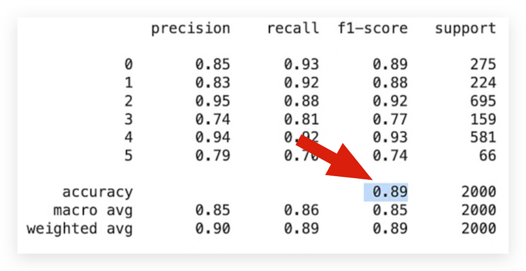
Notice the metrics — Precision and Recall.
They are quite close, which is excellent. This is exactly what we want. The final accuracy is 0.89, as shown in the Classification Report.
# 131. Print Confusion Matrix
print(confusion_matrix(y_test_le, predicted_labels))
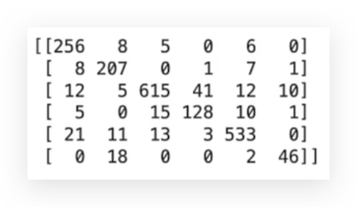
# 132. Print Accuracy Score
print(accuracy_score(y_test_le, predicted_labels))

# -----> 0.8925
And then, we reached an accuracy of 0.89 at the end.
After that, I saved the model to disk:
# 133. Save the Model in TensorFlow Format
model_v3.save("model_v3.keras")
Soon, I’ll make the comparison of the three versions, but before that, let’s do the deploy of the model from version 3.
Let’s go through the full process, from start to finish.
20. Model V3 — Deploy of the Fine-Tuned Model
Let’s proceed with the deploy of the model from version 3.
There’s a little issue with TensorFlow, as you know — there’s always some problem along the way.
TensorFlow doesn’t automatically recognize custom layers or objects that are not part of the core Keras TensorFlow library, such as the TFDistilBertModel. It doesn't recognize the layer, but it's a simple fix.
# 134. Load the Model

# 134.a Imports
from transformers import TFDistilBertModel
from tensorflow.keras.models import load_model
from tensorflow.keras.utils import custom_object_scope

# 134.b Load the model with the custom layer registered
reloaded_model = load_model(
    "model_v3.keras",
    custom_objects={"TransformerLayer": TransformerLayer}
)
So, I need to register this custom layer before loading the model from disk, okay? That’s what I’m doing here — I’m importing exactly the two necessary functions, and I’m specifying that I want an optimized object in this scope.
From there, I load the version 3 model, which we had already saved.
At this point, it will load the model back from disk into memory.
From here, the process is the same as in versions 1 and 2. So, I’ll prepare the sentences and use the same sentence from the previous versions.
# 135. New Sentence (Sentiment = Fear)
sentence = "i even feel a little shaky"
I construct the DataFrame:
# 136. Create a DataFrame with the Sentence
df_new = pd.DataFrame({'Sentence': [sentence]})
Then, I apply the preprocessing with Spacy:
# 137. Apply the Preprocessing Function
df_new['Processed_Sentence'] = df_new['Sentence'].apply(preprocess_text)
Next, I apply the encode.
Pay attention to the pattern — always pay close attention to the pattern:
# 138. Encode the New Data
new_data = encode_texts(
df_new['Processed_Sentence'], fast_tokenizer, maxlen=max_length)
I created three different versions of the model, and in all three, I followed the same pattern. What was that pattern?
Any processing applied to the training data must also be applied to new data and test data, as we did. In this case, these are new data, so I need to apply the encoding, just as we did with the training data.
So, I apply the encode using the fast_tokenizer and the maximum length, preparing the new data.
After that, I present the new data to the model and get the predictions:
# 139. Make Predictions with the Loaded Model
predictions = model_v3.predict(new_data)
Then, I retrieve the prediction with the highest probability:
# 140. Select the Class with the Highest Probability
highest_prob_class = np.argmax(predictions, axis=1)

# 141. Display the Class with the Highest Probability
highest_prob_class

# -----> array([4])
Then, I present this to you, but you don’t want the number 4.
You want the class name:
# 142. Get the Class Name
class_name = label_encoder_v3.inverse_transform(highest_prob_class)
So, I fetch this from our encoder, which is label_encoder_v3, and then we check the class name:
# 143. Predicted Class
class_name

So, I fetch this from our encoder, which is label_encoder_v3, and then we check the class name:
# 144. Disable Parallelism in the Transformers Package
%env TOKENIZERS_PARALLELISM=false
Let’s conclude this by doing a general comparison of the three versions of the model we’ve created so far.
Conclusion of the 3 Model Versions
Based on what we’ve discussed and the comparisons we’ve made between the three versions, the choice of the ideal model depends directly on the use case.
For this specific case, text sentiment classification, the simplest and fastest version, Version 1, is the best choice. While it has slightly lower accuracy, its simplicity, training speed, and ease of handling make it ideal for scenarios where high precision is not critical for the application.
Additionally, Version 1 is easier to fine-tune when necessary, which can be a significant benefit for production applications.
If we were dealing with situations where precision is crucial, such as classifying diseases in a medical context, choosing Version 3 would make more sense, given that it offers the highest accuracy. The impact of a wrong decision in such contexts can be significant, making Version 3 the best option for high-stakes scenarios.
Ultimately, the key is always to adapt the solution to the specific problem you’re trying to solve. In many cases, a simpler and faster model may be more effective, while in others, the higher complexity and precision of advanced models like Transformers are justified.
With that, we conclude the project, where we explored training three different versions of deep learning models for text sentiment classification, covering everything from model selection to deployment and performance evaluation.
Each version had its advantages, and the decision on which to use undoubtedly depends on the project’s context and requirements.
Thank you for following along! 🐼❤️
All images, content, and text by Leo Anello.
Bibliography and Useful Links:
1. GitHub Repository (Notebook)
2. Hugging Face
3. TensorFlow
4. BERT Paper
5. Spacy
6. DistilBERT
7. Adam Optimizer
8. Fine-Tuning Guide
Sentiment Analysis with Transformers: A Complete Deep Learning Project — PT. II was originally published in Towards Data Science on Medium, where people are continuing the conversation by highlighting and responding to this story.
from Datascience in Towards Data Science on Medium https://ift.tt/SG1B08y
via IFTTT


